ernanhughes
+++ date = ‘2025-01-18T16:38:07Z’ title = ‘Cellular Automata: Traffic Flow Simulation using the Nagel-Schreckenberg Model’ categories = [‘ca’] tag = [‘ca’] +++
Summary
The Nagel-Schreckenberg (NaSch) model is a traffic flow model which uses used cellular automata to simulate and predict traffic on roads.
Design of the Nagel-Schreckenberg Model
- Discrete Space and Time:
- The road is divided into cells, each representing a fixed length (e.g., a few meters).
- Time advances in discrete steps.
- Vehicle Representation:
- Each cell is either empty or occupied by a single vehicle.
- Each vehicle has a velocity (an integer) which determines how many cells it moves in a single time step.
Rules of the Model:
- The NaSch model uses local rules to update the state of each vehicle at every time step. These rules are:
- Acceleration:
- A vehicle increases its velocity by 1 unit (up to a maximum velocity (v_{\text{max}})).
- Deceleration:
- If the distance to the next vehicle ahead is less than the current velocity, the vehicle slows down to avoid a collision.
- Randomization:
- With a probability (p), a vehicle randomly decreases its velocity by 1 unit to account for driver imperfections or road conditions.
- Movement:
- Each vehicle moves forward by the updated velocity.
- Parameters:
- Road length: Total number of cells.
- Vehicle density: Fraction of cells occupied by vehicles.
- Maximum velocity ((v_{\text{max}})): Maximum speed of the vehicles.
- Randomization probability ((p)): Likelihood of a vehicle slowing down randomly.
Steps in the Simulation
- Initialization:
- Place vehicles on the road randomly or with a specific density.
- Assign each vehicle an initial velocity (often 0).
- Iterative Updates:
- For each time step, apply the four rules (acceleration, deceleration, randomization, and movement) to update the positions and velocities of all vehicles.
- Observation:
- Measure traffic metrics like flow, density, and average velocity to analyze traffic behavior under different conditions.
Python Implementation
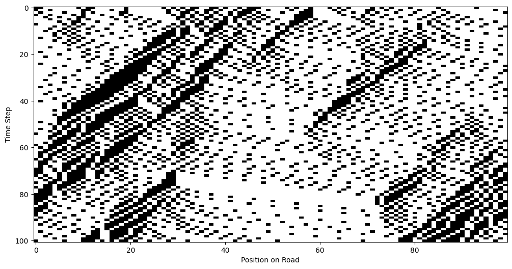
This python code will generate a road and show traversal along that road using the model.
import numpy as np
import matplotlib.pyplot as plt
from IPython.display import HTML

# Simulation parameters
road_length = 100  # Length of the road (number of cells)
num_cars = 30  # Number of cars on the road
max_speed = 5  # Maximum speed of cars (cells per time step)
p_slow = 0.3  # Probability of random slowing down
num_steps = 100  # Number of time steps to simulate

# road: An array representing the road where -1 indicates an empty cell.
# Initialize the road with empty cells (-1)
road = np.full(road_length, -1)

# Randomly place cars on the road with random initial speeds
car_positions = np.random.choice(road_length, num_cars, replace=False)
# Random initial speeds assigned to each car.
initial_speeds = np.random.randint(0, max_speed + 1, num_cars)
road[car_positions] = initial_speeds


def update_road(road):
    new_road = np.full_like(road, -1)
    road_length = len(road)
    for i in range(road_length):
        if road[i] != -1:
            speed = road[i]
            # Step 1: Acceleration
            if speed < max_speed:
                speed += 1
            # Step 2: Slowing down due to other cars
            distance = 1
            while distance <= speed and road[(i + distance) % road_length] == -1:
                distance += 1
            distance -= 1
            speed = min(speed, distance)
            # Step 3: Randomization
            if speed > 0 and np.random.rand() < p_slow:
                speed -= 1
            # Step 4: Move the car
            new_position = (i + speed) % road_length
            new_road[new_position] = speed
    return new_road


# Store the history of the road for visualization
road_history = [road.copy()]
for step in range(num_steps):
    road = update_road(road)
    road_history.append(road.copy())


# Prepare the figure
fig, ax = plt.subplots(figsize=(12, 6))
ax.set_xlabel("Position on Road")
ax.set_ylabel("Time Step")

# Convert road history to a 2D array for visualization
road_display = []
for state in road_history:
    display_state = np.where(state >= 0, 1, 0)  # 1 for car, 0 for empty
    road_display.append(display_state)
road_display = np.array(road_display)

# Display the simulation as an image
im = ax.imshow(road_display, cmap="Greys", interpolation="none", aspect="auto")

print(
    """Explanation: We create a 2D array where rows represent time steps and columns represent positions on the road.
         A value of 1 indicates a car, and 0 indicates an empty cell.
         We then use imshow to display this array as an image.
         We then save the traverse of the road as an animated gif and show that."""
)

# Show the generated road plot
plt.show()

image_filenames = []
for i, r in enumerate(road_display):
    ax.clear()
    ax.imshow([r], cmap="Greys", aspect="auto")
    ax.set_title(f"Time Step {i}")
    ax.set_xlabel("Position on Road")
    ax.set_yticks([])
    save_path = f"traffic_{i}.png"
    fig.savefig(save_path, dpi=300)
    image_filenames.append(save_path)


def create_gif(image_filenames, output_filename="traffic.gif", fps=2):
    """
    Creates an animated GIF from a list of image filenames.
    """
    from PIL import Image

    images = [Image.open(filename) for filename in image_filenames]
    images[0].save(
        output_filename,
        save_all=True,
        append_images=images[1:],
        duration=1000 // fps,
        loop=0,
    )

create_gif(image_filenames, output_filename="traffic.gif", fps=2)

from IPython.display import Image
Image(filename="traffic.gif")
The map
Traversal
Traffic Flow Dynamics
The NaSch model reproduces key traffic phenomena, including:
- Free Flow: At low vehicle densities, vehicles travel at their maximum velocity without interference.
- Congested Flow: At higher densities, vehicles form clusters, leading to slower movement and stop-and-go traffic.
- Jam Formation: With very high densities, vehicles are nearly stationary, forming traffic jams.
Applications of the NaSch Model
- Traffic Management:
- Predict traffic congestion under varying densities and road conditions.
- Evaluate the effects of traffic control measures (e.g., speed limits or lane closures).
- Urban Planning:
- Model the impact of new road networks or infrastructure changes on traffic flow.
- Driver Behavior Analysis:
- Incorporate different probabilities (p) to study the effects of driver aggressiveness or cautiousness.
- Autonomous Vehicles:
- Test traffic flow patterns in mixed environments with autonomous and human-driven vehicles.
Strengths and Limitations
Strengths:
- Simple and computationally efficient.
- Captures realistic traffic dynamics like free flow, congestion, and jams.
- Flexible for extensions (e.g., multi-lane roads or variable (v_{\text{max}})).
Limitations:
- Simplistic representation of vehicle and road dynamics.
- Does not account for detailed vehicle interactions like lane-changing or acceleration profiles.
- Randomization oversimplifies driver behavior.
Code Examples
Check out the ca notebooks for the code used in this post and additional examples.