ernanhughes

+++ date = ‘2025-01-18T03:03:36Z’ draft = true title = ‘Cellular Automata: Simulate Gastropod Shell Growth Using Cellular Automata’ +++

Summary

I started with this paper A developmentally descriptive method forquantifying shape in gastropod shells and bridged the results to a cellular automata approach.

An example of the shell we are modelling:

Steps

1. Identify the Key Biological Features

The paper outlines the logarithmic helicospiral model for shell growth, where:

• The shell grows outward and upward in a spiral shape.
• Parameters like width growth ((g_w)), height growth ((g_h)), and aperture shape dictate the final form.

These features describe how the shell expands over time in a predictable geometric pattern.

---

2. Translate the Features into Cellular Automata Concepts

Cellular automata are grid-based systems where cells evolve based on rules. To model the shell:

• Grid Representation: A 2D or 3D grid represents the space where the shell grows.
• Growth Rules:
  • Use a logarithmic equation to determine how cells (representing parts of the shell) activate and expand.
  • The growth follows the paper’s helicospiral formula: [ (x, y, z) = \left( r_0 e^{g_w t} \cos(t), -r_0 e^{g_w t} \sin(t), -h_0 e^{g_h t} \right) ]
  • This ensures the cells follow the natural spiral growth pattern.

---

3. Implement the Cellular Automata

• Cell States:
  • Cells are either active (part of the shell) or inactive (empty space).
  • Growth happens probabilistically or deterministically based on the spiral’s geometry.
• Time Evolution:
  • Cells activate over time based on their neighbors and the growth rules derived from the helicospiral.

---

4. Visualize the Growth

We visualized the shell formation:

• 2D Grid Approach:
  • A basic 2D representation shows how the spiral expands step by step.
• 3D Representation:
  • Polar coordinates and height were used to create a helicospiral in 3D, closer to the paper’s description.

---

import numpy as np
import matplotlib.pyplot as plt
from matplotlib.animation import PillowWriter
from PIL import Image

# Parameters
growth_rate_w = 0.2  # Controls spiral width
growth_rate_h = 0.1  # Controls spiral height
angle_step = 0.1  # Controls angular resolution
time_steps = 200  # Total steps in simulation

# Function to generate shell points in polar coordinates
def generate_shell_points(growth_rate_w, growth_rate_h, time_steps, angle_step):
    theta = np.arange(0, time_steps * angle_step, angle_step)  # Angular values
    r = np.exp(growth_rate_w * theta)  # Radial distance
    h = -growth_rate_h * theta  # Height decreases with angle
    return theta, r, h

# Function to plot the shell
def plot_shell(theta, r, h, step, save_path=None):
    x = r * np.cos(theta)
    y = r * np.sin(theta)
    fig = plt.figure(figsize=(8, 8))
    ax = fig.add_subplot(111, projection='3d')
    ax.plot(x, y, h, color='brown', lw=2)
    ax.set_title(f"Shell Growth Step {step}")
    ax.set_xlabel("X")
    ax.set_ylabel("Y")
    ax.set_zlabel("Height")
    ax.grid(False)
    ax.axis('off')
    if save_path:
        plt.savefig(save_path, dpi=300)
    plt.close(fig)

# Generate points for the shell
theta, r, h = generate_shell_points(growth_rate_w, growth_rate_h, time_steps, angle_step)

# Save each step as an image for GIF creation
images = []
for step in range(1, len(theta)):
    plot_shell(theta[:step], r[:step], h[:step], step, save_path=f"shell_step_{step}.png")
    images.append(Image.open(f"shell_step_{step}.png"))

# Create an animated GIF
gif_path = "realistic_shell_growth.gif"
images[0].save(
    gif_path, save_all=True, append_images=images[1:], duration=50, loop=0
)

from IPython.display import Image
Image(filename=gif_path)

This generates the following image

---

Key Advantages of Using Cellular Automata

1. Modularity:
   • CAs allow for easily modifying growth rules to experiment with different shell forms.
2. Emergent Behavior:
   • The complex spiral structure naturally emerges from simple growth rules.
3. Simulation Flexibility:
   • Parameters like (g_w) and (g_h) can be tuned to mimic various gastropod species.

---

Improving the image we generate

Add Cross Sections

1. Define the Aperture Shape:
   • Use geometric shapes (e.g., circles, ellipses, or custom curves) to represent the cross-section of the shell at each point along the spiral.
2. Extrude the Aperture:
   • Place these cross-sections along the spiral path and orient them perpendicularly to the curve.
3. Fill the Surface:
   • Connect the cross-sections to form a smooth, filled surface that resembles a natural shell.

---

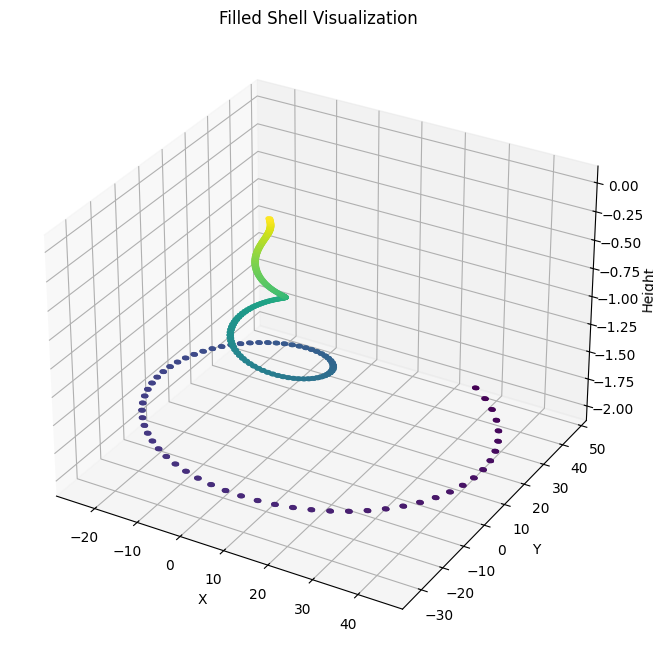
Filled Shell Visualization

import numpy as np
import matplotlib.pyplot as plt
from mpl_toolkits.mplot3d import Axes3D

# Parameters
growth_rate_w = 0.2  # Controls spiral width
growth_rate_h = 0.1  # Controls spiral height
angle_step = 0.1  # Angular resolution
time_steps = 200  # Total steps in simulation
aperture_radius = 0.5  # Radius of the circular cross-section

# Function to generate shell points with cross-sections
def generate_filled_shell(growth_rate_w, growth_rate_h, time_steps, angle_step, aperture_radius):
    theta = np.arange(0, time_steps * angle_step, angle_step)  # Angular values
    r = np.exp(growth_rate_w * theta)  # Radial distance
    h = -growth_rate_h * theta  # Height decreases with angle

    # Generate cross-sectional points (circle) for each step
    shell_points = []
    for t, radius, height in zip(theta, r, h):
        x_center = radius * np.cos(t)
        y_center = radius * np.sin(t)
        
        # Generate circular cross-section points
        cross_section = [
            (x_center + aperture_radius * np.cos(a),
             y_center + aperture_radius * np.sin(a),
             height)
            for a in np.linspace(0, 2 * np.pi, 20)
        ]
        shell_points.extend(cross_section)
    return np.array(shell_points)

# Generate the filled shell
shell_points = generate_filled_shell(
    growth_rate_w, growth_rate_h, time_steps, angle_step, aperture_radius
)

# Plot the filled shell
fig = plt.figure(figsize=(10, 8))
ax = fig.add_subplot(111, projection='3d')

# Extract coordinates
x, y, z = shell_points[:, 0], shell_points[:, 1], shell_points[:, 2]

# Scatter plot with small points to visualize the filled structure
ax.scatter(x, y, z, s=1, c=z, cmap='viridis', alpha=0.8)

# Set plot aesthetics
ax.set_title("Filled Shell Visualization")
ax.set_xlabel("X")
ax.set_ylabel("Y")
ax.set_zlabel("Height")
plt.show()

Key Changes

1. Polar to Cartesian Conversion:
   • Shell points are generated in polar coordinates ((r, \theta)) and then converted to Cartesian coordinates ((x, y)).
2. Height and Growth Rates:
   • The height (h) and radial growth (r) are tied to angular progress (\theta), creating a helicospiral.
3. 3D Visualization:
   • The shell is plotted in 3D, capturing its natural spiral structure.
4. Improved Aesthetics:
   • The color and thickness of the line, as well as the 3D perspective, mimic the appearance of real shells.

---

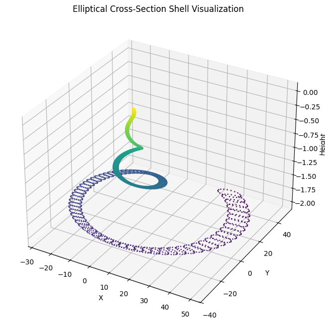
Updated Code for Elliptical Cross-Sections

import numpy as np
import matplotlib.pyplot as plt
from mpl_toolkits.mplot3d import Axes3D

# Parameters
growth_rate_w = 0.2  # Controls spiral width
growth_rate_h = 0.1  # Controls spiral height
angle_step = 0.1  # Angular resolution
time_steps = 200  # Total steps in simulation
base_aperture_width = 0.5  # Base width of the cross-section (ellipse)
base_aperture_height = 0.2  # Base height of the cross-section (ellipse)
aperture_scaling = 0.1  # Scaling factor for aperture growth

# Function to generate shell points with elliptical cross-sections
def generate_elliptical_shell(growth_rate_w, growth_rate_h, time_steps, angle_step,
                              base_aperture_width, base_aperture_height, aperture_scaling):
    theta = np.arange(0, time_steps * angle_step, angle_step)  # Angular values
    r = np.exp(growth_rate_w * theta)  # Radial distance
    h = -growth_rate_h * theta  # Height decreases with angle

    # Generate elliptical cross-sectional points for each step
    shell_points = []
    for t, radius, height in zip(theta, r, h):
        x_center = radius * np.cos(t)
        y_center = radius * np.sin(t)
        
        # Adjust aperture dimensions based on the radial distance
        aperture_width = base_aperture_width + aperture_scaling * radius
        aperture_height = base_aperture_height + aperture_scaling * radius * 0.5
        
        # Generate elliptical cross-section points
        cross_section = [
            (x_center + aperture_width * np.cos(a),
             y_center + aperture_height * np.sin(a),
             height)
            for a in np.linspace(0, 2 * np.pi, 20)
        ]
        shell_points.extend(cross_section)
    return np.array(shell_points)

# Generate the filled shell with elliptical cross-sections
elliptical_shell_points = generate_elliptical_shell(
    growth_rate_w, growth_rate_h, time_steps, angle_step,
    base_aperture_width, base_aperture_height, aperture_scaling
)

# Plot the shell with elliptical cross-sections
fig = plt.figure(figsize=(10, 8))
ax = fig.add_subplot(111, projection='3d')

# Extract coordinates
x, y, z = elliptical_shell_points[:, 0], elliptical_shell_points[:, 1], elliptical_shell_points[:, 2]

# Scatter plot with small points to visualize the filled structure
ax.scatter(x, y, z, s=1, c=z, cmap='viridis', alpha=0.8)

# Set plot aesthetics
ax.set_title("Elliptical Cross-Section Shell Visualization")
ax.set_xlabel("X")
ax.set_ylabel("Y")
ax.set_zlabel("Height")
plt.show()

---

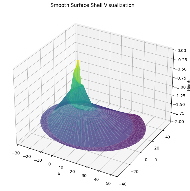
Smooth Surface Rendering

Replace scatter plots with a 3D surface for smoother visualization. We’ll interpolate the points between cross-sections and use a library like mpl_toolkits.mplot3d to render a surface.

from scipy.spatial import Delaunay

# Generate the 3D surface
fig = plt.figure(figsize=(10, 8))
ax = fig.add_subplot(111, projection='3d')

# Create a surface by triangulating the points
tri = Delaunay(elliptical_shell_points[:, :2])  # Use x and y coordinates for triangulation
ax.plot_trisurf(
    elliptical_shell_points[:, 0],  # X-coordinates
    elliptical_shell_points[:, 1],  # Y-coordinates
    elliptical_shell_points[:, 2],  # Z-coordinates
    triangles=tri.simplices, cmap="viridis", alpha=0.8
)

# Set plot aesthetics
ax.set_title("Smooth Surface Shell Visualization")
ax.set_xlabel("X")
ax.set_ylabel("Y")
ax.set_zlabel("Height")
plt.show()

---

Step 3: Texturing

We can add color patterns or gradients to simulate natural shell patterns. This involves mapping a texture (e.g., stripes or spots) onto the surface.

---

Updated Code for Texturing

# Define a texture pattern (striped bands)
def generate_texture(z):
    return np.sin(z * 10) * 0.5 + 0.5  # Stripe effect

# Apply the texture
fig = plt.figure(figsize=(10, 8))
ax = fig.add_subplot(111, projection='3d')

# Texture mapping
colors = generate_texture(elliptical_shell_points[:, 2])  # Use Z-coordinates for texture pattern
ax.scatter(
    elliptical_shell_points[:, 0],
    elliptical_shell_points[:, 1],
    elliptical_shell_points[:, 2],
    c=colors, cmap="copper", s=1, alpha=0.8
)

# Set plot aesthetics
ax.set_title("Textured Shell Visualization")
ax.set_xlabel("X")
ax.set_ylabel("Y")
ax.set_zlabel("Height")
plt.show()

---

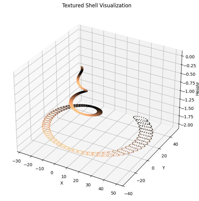
Summary of Enhancements

1. Elliptical Cross-Sections: Added realistic aperture shapes with width and height scaling.
2. Smooth Surface Rendering: Transitioned from scatter points to triangulated 3D surfaces.
3. Texturing: Applied color gradients or patterns to simulate natural shell designs.

Code Examples

Check out the shells notebook for the code used in this post.

Summary

Using cellular automata, we recreated the paper’s gastropod shell growth model by simulating the process of logarithmic helicospiral expansion. This approach transforms abstract biological principles into computational steps, enabling exploration, visualization, and experimentation with shell shapes in a flexible and intuitive way.