ernanhughes
+++ date = ‘2025-01-17T18:07:50Z’ draft = true title = ‘43 Machine Learning Questions and Answers with Python examples’ +++
1. What is overfitting, and how can you prevent it in machine learning?
Answer: Overfitting occurs when a model learns the noise and details in the training data to the extent that it negatively impacts the model’s performance on new data. It essentially “memorizes” the training data instead of learning the underlying patterns.
Prevention Methods:
- Cross-validation
- Regularization (L1, L2)
- Pruning (in decision trees)
- Early stopping (in neural networks)
- Increasing the amount of training data
Python Example:
from sklearn.datasets import make_classification
from sklearn.model_selection import train_test_split
from sklearn.linear_model import LogisticRegression
from sklearn.model_selection import cross_val_score

# Generate a toy classification dataset
X, y = make_classification(n_samples=1000, n_features=20, random_state=42)

# Split data into training and testing sets
X_train, X_test, y_train, y_test = train_test_split(X, y, test_size=0.2, random_state=42)

# Initialize the model
model = LogisticRegression(max_iter=10000)

# Perform cross-validation to check for overfitting
scores = cross_val_score(model, X_train, y_train, cv=5)
print(f'Cross-validation scores: {scores}')
print(f'Mean cross-validation score: {scores.mean()}')
Cross-validation scores: [0.85625 0.875   0.85625 0.86875 0.88125]
Mean cross-validation score: 0.8674999999999999
2. What is the difference between supervised and unsupervised learning?
Answer:
- Supervised Learning: The model is trained using labeled data, i.e., data with both input features and corresponding output labels. Examples: classification, regression.
- Unsupervised Learning: The model is trained on data that has no labeled responses. It tries to identify patterns or groupings in the data. Examples: clustering, dimensionality reduction.
Supervised Learning Example: Regression (Predicting House Prices)
In this example, we’ll use a simple linear regression model to predict house prices based on some features like the size of the house.
Python Code for Regression:
import numpy as np
import matplotlib.pyplot as plt
from sklearn.linear_model import LinearRegression
from sklearn.model_selection import train_test_split
from sklearn.datasets import make_regression

# Generate some synthetic data for regression (house size vs price)
X, y = make_regression(n_samples=100, n_features=1, noise=10, random_state=42)

# Split the data into training and testing sets
X_train, X_test, y_train, y_test = train_test_split(X, y, test_size=0.2, random_state=42)

# Initialize the Linear Regression model
model = LinearRegression()

# Train the model on the training data
model.fit(X_train, y_train)

# Make predictions on the test set
y_pred = model.predict(X_test)

# Plot the results
plt.scatter(X_test, y_test, color='blue', label='Actual Prices')
plt.plot(X_test, y_pred, color='red', label='Predicted Prices')
plt.title('Regression: House Price Prediction')
plt.xlabel('House Size (sq ft)')
plt.ylabel('Price ($)')
plt.legend()
plt.show()

# Print model performance
print(f'Model Coefficients: {model.coef_}')
print(f'Model Intercept: {model.intercept_}')
Results
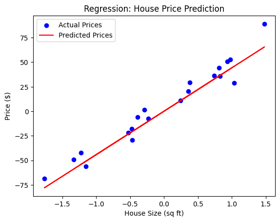
Explanation:
- We use
make_regressionto generate synthetic data where the target (y) is a continuous variable (house price), and the feature (X) is the size of the house. - We split the dataset into training and testing sets using
train_test_split. - We train a Linear Regression model and make predictions on the test set.
- Finally, we plot the actual prices and the predicted prices for comparison.
Supervised Learning Example: Classification (Iris Flower Classification)
In this example, we’ll use the k-Nearest Neighbors (k-NN) classifier to classify the species of an iris flower based on its features.
Python Code for Classification:
from sklearn.datasets import load_iris
from sklearn.model_selection import train_test_split
from sklearn.neighbors import KNeighborsClassifier
from sklearn.metrics import accuracy_score

# Load the Iris dataset
iris = load_iris()
X, y = iris.data, iris.target

# Split the data into training and testing sets
X_train, X_test, y_train, y_test = train_test_split(X, y, test_size=0.3, random_state=42)

# Initialize the k-NN classifier
knn = KNeighborsClassifier(n_neighbors=3)

# Train the classifier on the training data
knn.fit(X_train, y_train)

# Make predictions on the test set
y_pred = knn.predict(X_test)

# Evaluate the model performance
print(f'Accuracy: {accuracy_score(y_test, y_pred)}')

# Show the classification results
print(f'Predicted Classes: {y_pred}')
print(f'Actual Classes: {y_test}')
Accuracy: 1.0
Predicted Classes: [1 0 2 1 1 0 1 2 1 1 2 0 0 0 0 1 2 1 1 2 0 2 0 2 2 2 2 2 0 0 0 0 1 0 0 2 1
 0 0 0 2 1 1 0 0]
Actual Classes: [1 0 2 1 1 0 1 2 1 1 2 0 0 0 0 1 2 1 1 2 0 2 0 2 2 2 2 2 0 0 0 0 1 0 0 2 1
 0 0 0 2 1 1 0 0]
Explanation:
- We load the Iris dataset from
sklearn.datasets, which contains data on different species of iris flowers. - The target variable
yrepresents the species, whileXcontains the features (sepal length, sepal width, petal length, and petal width). - We use the k-NN classifier to train the model and predict the species of flowers in the test set.
- The model’s performance is evaluated using accuracy.
Key Differences Between Regression and Classification:
- Regression:
- Predicts continuous numerical values.
- Example: Predicting house prices.
- Common models: Linear Regression, Decision Trees (for regression), Random Forest (for regression).
- Classification:
- Predicts discrete class labels.
- Example: Classifying flowers into species.
- Common models: Logistic Regression, k-NN, Support Vector Machines (SVM), Decision Trees (for classification), Random Forest (for classification).
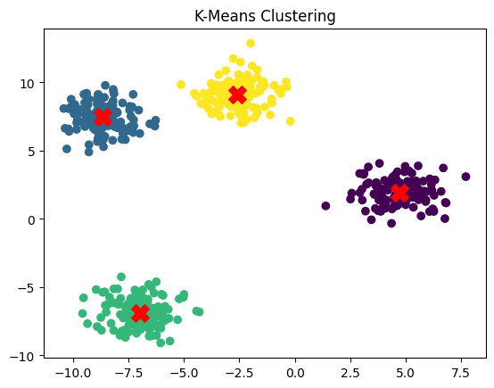
Unsupervised Learning example: Clustering with K-Means:
from sklearn.datasets import make_blobs
from sklearn.cluster import KMeans
import matplotlib.pyplot as plt

# Create a toy dataset for clustering
X, _ = make_blobs(n_samples=500, centers=4, random_state=42)

# Apply KMeans clustering
kmeans = KMeans(n_clusters=4, random_state=42)
y_kmeans = kmeans.fit_predict(X)

# Visualize the clusters
plt.scatter(X[:, 0], X[:, 1], c=y_kmeans, cmap='viridis')
plt.scatter(kmeans.cluster_centers_[:, 0], kmeans.cluster_centers_[:, 1], s=200, c='red', marker='X')
plt.title("K-Means Clustering")
plt.show()
3. What is cross-validation, and why is it important?
Answer: Cross-validation is a technique used to evaluate the performance of a machine learning model by partitioning the data into multiple subsets (folds). The model is trained on some folds and tested on the remaining fold, and this process is repeated several times to obtain an average performance score.
Why is it important? It helps to reduce overfitting, gives a more reliable estimate of model performance, and makes better use of limited data.
Python Example:
from sklearn.model_selection import cross_val_score
from sklearn.ensemble import RandomForestClassifier
from sklearn.datasets import load_iris

# Load dataset
X, y = load_iris(return_X_y=True)

# Initialize the model
model = RandomForestClassifier()

# Perform cross-validation
scores = cross_val_score(model, X, y, cv=5)
print(f'Cross-validation scores: {scores}')
print(f'Mean accuracy: {scores.mean()}')
Results
Cross-validation scores: [0.96666667 0.96666667 0.93333333 0.96666667 1.        ]
Mean accuracy: 0.9666666666666668
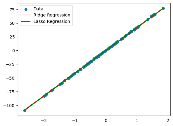
4. What is regularization, and what types of regularization are commonly used?
Answer: Regularization is a technique used to prevent overfitting by adding a penalty term to the model’s loss function. It discourages the model from fitting overly complex models that may overfit the data.
- L1 Regularization (Lasso): Adds the absolute value of the coefficients to the loss function.
- L2 Regularization (Ridge): Adds the squared value of the coefficients to the loss function.
Python Example:
from sklearn.linear_model import Ridge, Lasso
from sklearn.datasets import make_regression
import matplotlib.pyplot as plt

# Generate a regression dataset
X, y = make_regression(n_samples=100, n_features=1, noise=0.5, random_state=42)

# Fit Ridge and Lasso models with regularization
ridge = Ridge(alpha=1.0)
lasso = Lasso(alpha=0.1)

ridge.fit(X, y)
lasso.fit(X, y)

# Plot the results
plt.scatter(X, y, label='Data')
plt.plot(X, ridge.predict(X), label='Ridge Regression', color='r')
plt.plot(X, lasso.predict(X), label='Lasso Regression', color='g')
plt.legend()
plt.show()
5. What is the bias-variance tradeoff?
Answer: The bias-variance tradeoff is the balance between two sources of error that affect machine learning models:
- Bias: Error due to overly simplistic models (underfitting).
- Variance: Error due to overly complex models (overfitting).
The goal is to find a model that generalizes well and has low bias and variance.
Python Example:
from sklearn.datasets import make_classification
from sklearn.model_selection import train_test_split
from sklearn.linear_model import LogisticRegression
from sklearn.tree import DecisionTreeClassifier
from sklearn.metrics import accuracy_score

# Generate a simple classification dataset
X, y = make_classification(n_samples=1000, n_features=20, random_state=42)

# Split into training and testing sets
X_train, X_test, y_train, y_test = train_test_split(X, y, test_size=0.2, random_state=42)

# Logistic Regression (high bias, low variance)
logreg = LogisticRegression()
logreg.fit(X_train, y_train)
y_pred_logreg = logreg.predict(X_test)
logreg_accuracy = accuracy_score(y_test, y_pred_logreg)

# Decision Tree (low bias, high variance)
dtree = DecisionTreeClassifier()
dtree.fit(X_train, y_train)
y_pred_dtree = dtree.predict(X_test)
dtree_accuracy = accuracy_score(y_test, y_pred_dtree)

print(f"Logistic Regression accuracy: {logreg_accuracy}")
print(f"Decision Tree accuracy: {dtree_accuracy}")
Logistic Regression accuracy: 0.855
Decision Tree accuracy: 0.845
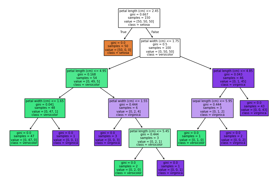
6. What are decision trees, and how do they work?
Answer: A decision tree is a supervised learning algorithm used for classification and regression. It splits the data into subsets based on the feature values, creating a tree-like structure of decisions and outcomes.
Python Example:
from sklearn.tree import DecisionTreeClassifier, plot_tree
from sklearn.datasets import load_iris

# Load dataset
X, y = load_iris(return_X_y=True)

# Fit a decision tree classifier
dtree = DecisionTreeClassifier(random_state=42)
dtree.fit(X, y)

# Plot the decision tree
plt.figure(figsize=(12, 8))
plot_tree(dtree, filled=True, feature_names=load_iris().feature_names, class_names=load_iris().target_names)
plt.show()
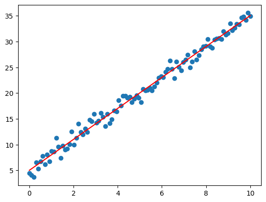
7. What is gradient descent?
Answer: Gradient descent is an optimization algorithm used to minimize the loss function by iteratively moving towards the minimum value of the function. It is widely used for training machine learning models, especially neural networks.
Python Example (Linear Regression):
import numpy as np
import matplotlib.pyplot as plt

# Generate some data
X = np.linspace(0, 10, 100)
y = 3 * X + 5 + np.random.randn(100)  # y = 3x + 5 with noise

# Initialize parameters
m = 0  # Slope (weight)
b = 0  # Intercept (bias)
learning_rate = 0.01
epochs = 1000

# Gradient Descent loop
for _ in range(epochs):
    y_pred = m * X + b
    error = y_pred - y
    m_gradient = (2 / len(X)) * np.dot(error, X)  # Derivative with respect to m
    b_gradient = (2 / len(X)) * np.sum(error)  # Derivative with respect to b
    m -= learning_rate * m_gradient
    b -= learning_rate * b_gradient

# Plotting the result
plt.scatter(X, y)
plt.plot(X, m * X + b, color='red')
plt.show()
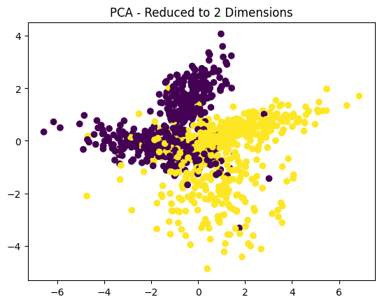
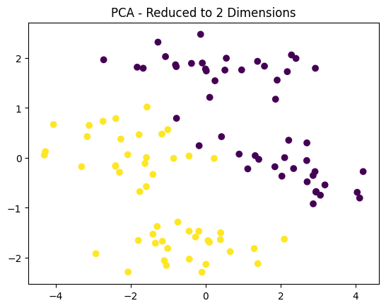
8. What is the “curse of dimensionality”?
Answer: The “curse of dimensionality” refers to the exponential increase in computational complexity and data sparsity as the number of features (dimensions) grows. In high-dimensional spaces, distances between data points become less meaningful, making clustering and classification algorithms less effective.
Python Example (PCA for Dimensionality Reduction):
from sklearn.decomposition import PCA
from sklearn.datasets import make_classification

# Create a high-dimensional dataset
X, y = make_classification(n_samples=1000, n_features=50, random_state=42)

# Apply PCA to reduce dimensions
pca = PCA(n_components=2)
X_reduced = pca.fit_transform(X)

# Plot the reduced data
plt.scatter(X_reduced[:, 0], X_reduced[:, 1], c=y, cmap='viridis')
plt.title("PCA - Reduced to 2 Dimensions")
plt.show()
9. How do you evaluate the performance of a classification model?
Answer: The performance of a classification model can be evaluated using several metrics, including:
- Accuracy: The proportion of correct predictions.
- Precision: The proportion of true positive predictions out of all positive predictions.
- Recall: The proportion of true positive predictions out of all actual positive instances.
- F1-Score: The harmonic mean of precision and recall.
- ROC-AUC: Measures the area under the ROC curve, showing the tradeoff between true positive rate and false positive rate.
Python Example:
from sklearn.metrics import classification_report
from sklearn.model_selection import train_test_split
from sklearn.linear_model import LogisticRegression
from sklearn.datasets import load_iris

# Load dataset
X, y = load_iris(return_X_y=True)

# Split the data
X_train, X_test, y_train, y_test = train_test_split(X, y, test_size=0.2, random_state=42)

# Train a model
model = LogisticRegression(max_iter=10000)
model.fit(X_train, y_train)

# Make predictions
y_pred = model.predict(X_test)

# Evaluate performance
print(classification_report(y_test, y_pred))
Classification Report
             precision    recall  f1-score   support

           0       1.00      1.00      1.00        10
           1       1.00      1.00      1.00         9
           2       1.00      1.00      1.00        11

    accuracy                           1.00        30
   macro avg       1.00      1.00      1.00        30
weighted avg       1.00      1.00      1.00        30
10. What is ensemble learning?
Answer: Ensemble learning is a technique where multiple models (often of the same type) are combined to make predictions, improving accuracy and robustness. Common ensemble methods include:
- Bagging (e.g., Random Forest)
- Boosting (e.g., XGBoost, AdaBoost)
- Stacking
Python Example (Random Forest):
from sklearn.ensemble import RandomForestClassifier
from sklearn.datasets import load_iris
from sklearn.model_selection import train_test_split
from sklearn.metrics import accuracy_score

# Load dataset
X, y = load_iris(return_X_y=True)

# Split into train and test sets
X_train, X_test, y_train, y_test = train_test_split(X, y, test_size=0.3, random_state=42)

# Train RandomForest model
rf = RandomForestClassifier(n_estimators=100)
rf.fit(X_train, y_train)

# Make predictions
y_pred = rf.predict(X_test)

# Evaluate the model
print(f"Accuracy: {accuracy_score(y_test, y_pred)}")
Accuracy: 1.0
11. What is the difference between classification and regression?
Answer:
- Classification: The task where the model predicts discrete labels or categories. Example: Predicting whether an email is spam or not.
- Regression: The task where the model predicts continuous numerical values. Example: Predicting house prices based on features like size and location.
Python Example (Classification and Regression):
# Classification example
from sklearn.datasets import load_iris
from sklearn.model_selection import train_test_split
from sklearn.linear_model import LogisticRegression
from sklearn.metrics import accuracy_score

X, y = load_iris(return_X_y=True)
X_train, X_test, y_train, y_test = train_test_split(X, y, test_size=0.3, random_state=42)

# Classification model
classifier = LogisticRegression(max_iter=10000)
classifier.fit(X_train, y_train)
y_pred_class = classifier.predict(X_test)
print(f'Classification Accuracy: {accuracy_score(y_test, y_pred_class)}')

# Regression example
from sklearn.datasets import make_regression
from sklearn.linear_model import LinearRegression

X_reg, y_reg = make_regression(n_samples=100, n_features=1, noise=0.1, random_state=42)
X_train_reg, X_test_reg, y_train_reg, y_test_reg = train_test_split(X_reg, y_reg, test_size=0.3, random_state=42)

# Regression model
regressor = LinearRegression()
regressor.fit(X_train_reg, y_train_reg)
y_pred_reg = regressor.predict(X_test_reg)
print(f'Regression R^2: {regressor.score(X_test_reg, y_test_reg)}')
Classification Accuracy: 1.0
Regression R^2: 0.9999930887851615
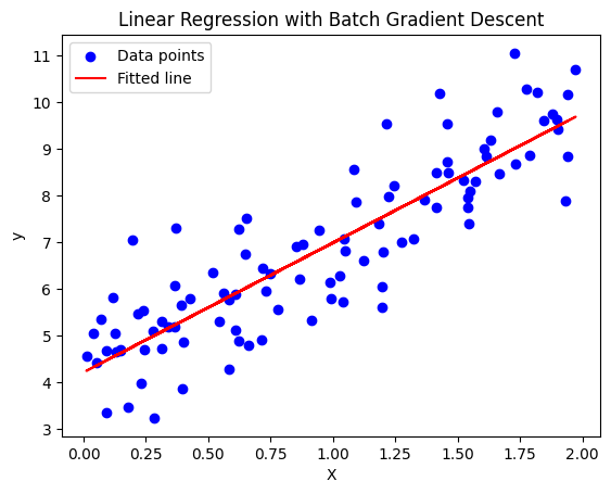
12. What are the different types of gradient descent algorithms?
Answer:
- Batch Gradient Descent: Computes the gradient using the entire dataset.
- Stochastic Gradient Descent (SGD): Computes the gradient using a single data point.
- Mini-Batch Gradient Descent: Computes the gradient using a subset (mini-batch) of the dataset.
Batch Gradient Descent Algorithm:
- Initialize the parameters (weights).
- Compute the prediction for all training data.
- Compute the cost function (mean squared error).
- Calculate the gradients of the cost function with respect to each parameter.
- Update the parameters (weights) by moving them in the direction of the negative gradient.
- Repeat the process until convergence (i.e., when the cost function stops changing significantly).
Python Code for Batch Gradient Descent:
import numpy as np
import matplotlib.pyplot as plt

# Generate synthetic data (y = 2 * X + 1 + noise)
np.random.seed(42)
X = 2 * np.random.rand(100, 1)  # Random feature between 0 and 2
y = 4 + 3 * X + np.random.randn(100, 1)  # y = 4 + 3X + noise

# Add an extra column of ones to X for the intercept (bias term)
X_b = np.c_[np.ones((100, 1)), X]  # Add x0 = 1 for each instance

# Hyperparameters
learning_rate = 0.1  # Learning rate
n_iterations = 1000  # Number of iterations
m = len(X_b)  # Number of training examples

# Initialize weights (parameters)
theta = np.random.randn(2, 1)  # Random initial weights

# Batch Gradient Descent
for iteration in range(n_iterations):
    # Compute the predictions
    predictions = X_b.dot(theta)

    # Compute the gradient of the cost function
    gradients = 2 / m * X_b.T.dot(predictions - y)

    # Update the weights (parameters) by subtracting the gradient
    theta -= learning_rate * gradients

# Print the final parameters (weights)
print(f"Final parameters (theta): {theta}")

# Make predictions using the learned parameters
y_pred = X_b.dot(theta)

# Plot the data and the fitted line
plt.scatter(X, y, color='blue', label='Data points')
plt.plot(X, y_pred, color='red', label='Fitted line')
plt.xlabel('X')
plt.ylabel('y')
plt.legend()
plt.title('Linear Regression with Batch Gradient Descent')
plt.show()
Explanation:
- Data Generation:
- We generate some synthetic data where the true relationship is (y = 4 + 3X + \text{noise}).
- Adding Bias Term:
- We add a column of ones to the feature matrix
Xto account for the intercept term (( \theta_0 )) in linear regression.
- We add a column of ones to the feature matrix
- Hyperparameters:
learning_rate: Determines how much we update the weights in each iteration.n_iterations: The number of iterations to run the gradient descent algorithm.
- Initialization:
- We initialize the weights (
theta) randomly. The size ofthetais 2, corresponding to the intercept term and the slope.
- We initialize the weights (
- Gradient Calculation:
- We calculate the gradients of the cost function with respect to the weights and update the weights by subtracting the learning rate times the gradient.
- Plotting:
- After running the gradient descent, we plot the original data points and the fitted line based on the learned parameters.
Key Concepts in the Code:
-
Cost Function: The cost function (mean squared error) measures how far the predicted values are from the actual values.
-
Gradient: The gradient is the partial derivative of the cost function with respect to each parameter. It tells us the direction to adjust the parameters to minimize the cost function.
-
Updating Weights: The weights (parameters) are updated in the direction opposite to the gradient (gradient descent), which leads to minimizing the cost function.
Output:
After running the code, the model learns the parameters, and the output should be close to the actual values (intercept = 4, slope = 3). The plot will show the data points and the fitted line based on the learned parameters.
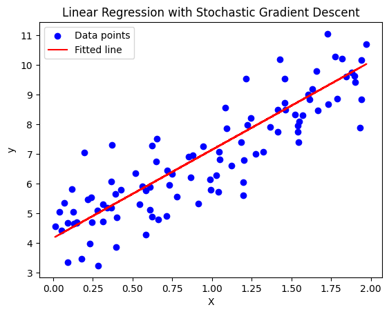
In Stochastic Gradient Descent, instead of computing the gradient for the entire dataset (as in Batch Gradient Descent), we compute the gradient using just a single data point at a time. This makes the updates faster, but more noisy. The model parameters are updated after each individual data point, rather than after the whole dataset.
Stochastic Gradient Descent for Linear Regression:
- Initialize the parameters (weights).
- For each training example:
- Make a prediction.
- Calculate the gradient of the loss with respect to the model parameters.
- Update the parameters using the gradient.
- Repeat the process for a specified number of epochs.
Python Code for Stochastic Gradient Descent:
import numpy as np
import matplotlib.pyplot as plt

# Generate synthetic data (y = 2 * X + 1 + noise)
np.random.seed(42)
X = 2 * np.random.rand(100, 1)  # Random feature between 0 and 2
y = 4 + 3 * X + np.random.randn(100, 1)  # y = 4 + 3X + noise

# Add an extra column of ones to X for the intercept (bias term)
X_b = np.c_[np.ones((100, 1)), X]  # Add x0 = 1 for each instance

# Hyperparameters
learning_rate = 0.1  # Learning rate
n_epochs = 50  # Number of epochs

# Initialize weights (parameters)
theta = np.random.randn(2, 1)  # Random initial weights

# Stochastic Gradient Descent
for epoch in range(n_epochs):
    for i in range(len(X_b)):
        # Pick a random data point
        xi = X_b[i:i+1]
        yi = y[i:i+1]

        # Compute the prediction
        prediction = xi.dot(theta)

        # Compute the gradient
        gradients = 2 * xi.T.dot(prediction - yi)

        # Update the parameters
        theta -= learning_rate * gradients

# Print the final parameters (weights)
print(f"Final parameters (theta): {theta}")

# Make predictions using the learned parameters
y_pred = X_b.dot(theta)

# Plot the data and the fitted line
plt.scatter(X, y, color='blue', label='Data points')
plt.plot(X, y_pred, color='red', label='Fitted line')
plt.xlabel('X')
plt.ylabel('y')
plt.legend()
plt.title('Linear Regression with Stochastic Gradient Descent')
plt.show()
Explanation of the Code:
- Data Generation:
- We generate synthetic data where the true relationship is ( y = 4 + 3X + \text{noise} ). This is just a simple linear regression task with some noise added.
- Feature Matrix:
- We add a column of ones to
Xto account for the intercept term (( \theta_0 )) in linear regression. This is done by creatingX_b.
- We add a column of ones to
- Hyperparameters:
learning_rate: The step size for each update.n_epochs: The number of iterations over the entire dataset.
- Parameter Initialization:
- We initialize the parameters (
theta) randomly. These represent the weights (slope and intercept) of our linear model.
- We initialize the parameters (
- Stochastic Gradient Descent:
- For each epoch (iteration over the data), we loop over each data point (i.e., each
xiandyi). - For each data point, we compute the prediction and the gradient.
- We update the parameters using the computed gradient and the learning rate.
- For each epoch (iteration over the data), we loop over each data point (i.e., each
- Final Parameters:
- After all iterations, the model has learned the parameters that minimize the error between predictions and actual values. We print the final learned parameters.
- Visualization:
- We plot the original data points and the fitted line based on the learned parameters.
Why Stochastic Gradient Descent?
- Efficiency: For large datasets, Batch Gradient Descent can be computationally expensive since it requires processing the entire dataset for each update. In contrast, SGD updates the parameters after seeing each individual data point, making it faster and more efficient for large datasets.
- Noisy Updates: Each update is based on a single data point, making the updates noisy. However, this often helps escape local minima in complex loss functions.
Output:
- The final model parameters (
theta) will be printed. In this case, the model should learn values close to the true parameters, which are ( \theta_0 = 4 ) (intercept) and ( \theta_1 = 3 ) (slope). - A plot will be shown with the original data points and the fitted regression line.
SGD and Mini-Batch Gradient Descent:
from sklearn.linear_model import SGDRegressor
from sklearn.datasets import make_regression
from sklearn.model_selection import train_test_split

# Generate regression data
X, y = make_regression(n_samples=100, n_features=1, noise=0.1, random_state=42)

# Split data
X_train, X_test, y_train, y_test = train_test_split(X, y, test_size=0.3, random_state=42)

# Stochastic Gradient Descent
sgd = SGDRegressor(max_iter=1000)
sgd.fit(X_train, y_train)
print(f'SGD R^2: {sgd.score(X_test, y_test)}')
SGD R^2: 0.9999836978386981
13. What is the difference between bagging and boosting?
Answer:
- Bagging (Bootstrap Aggregating): Involves training multiple models on different random subsets of the training data, then averaging their predictions (e.g., Random Forest).
- Boosting: Involves training multiple models sequentially, where each new model corrects the errors made by the previous one (e.g., AdaBoost, XGBoost).
Python Example (Random Forest for Bagging and AdaBoost for Boosting):
from sklearn.ensemble import RandomForestClassifier, AdaBoostClassifier
from sklearn.datasets import load_iris
from sklearn.model_selection import train_test_split
from sklearn.metrics import accuracy_score

# Load dataset
X, y = load_iris(return_X_y=True)
X_train, X_test, y_train, y_test = train_test_split(X, y, test_size=0.3, random_state=42)

# Bagging with Random Forest
rf = RandomForestClassifier(n_estimators=100)
rf.fit(X_train, y_train)
y_pred_rf = rf.predict(X_test)
print(f'Random Forest (Bagging) Accuracy: {accuracy_score(y_test, y_pred_rf)}')

# Boosting with AdaBoost
ab = AdaBoostClassifier(n_estimators=100)
ab.fit(X_train, y_train)
y_pred_ab = ab.predict(X_test)
print(f'AdaBoost (Boosting) Accuracy: {accuracy_score(y_test, y_pred_ab)}')
Random Forest (Bagging) Accuracy: 1.0
AdaBoost (Boosting) Accuracy: 1.0
14. What is the purpose of the activation function in neural networks?
Answer: The activation function introduces non-linearity into the network, enabling it to learn complex patterns. Without an activation function, the network would behave like a linear regression model, no matter how many layers it has.
Common activation functions:
- ReLU (Rectified Linear Unit)
- Sigmoid
- Tanh
Python Example (Neural Network with ReLU):
from sklearn.datasets import make_classification
from sklearn.model_selection import train_test_split
from sklearn.neural_network import MLPClassifier
from sklearn.metrics import accuracy_score

# Generate classification dataset
X, y = make_classification(n_samples=1000, n_features=20, random_state=42)

# Split the data
X_train, X_test, y_train, y_test = train_test_split(X, y, test_size=0.3, random_state=42)

# Neural network model with ReLU activation
model = MLPClassifier(hidden_layer_sizes=(50,), activation='relu', max_iter=1000)
model.fit(X_train, y_train)

# Predict and evaluate the model
y_pred = model.predict(X_test)
print(f'Neural Network Accuracy: {accuracy_score(y_test, y_pred)}')
Neural Network Accuracy: 0.8333333333333334
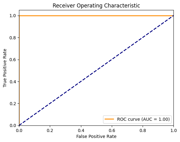
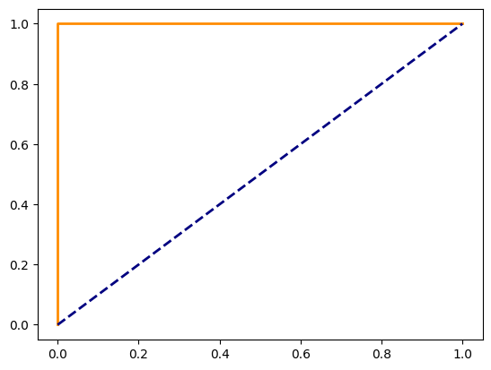
15. What is the ROC curve, and how do you interpret it?
Answer: The Receiver Operating Characteristic (ROC) curve is a graphical representation of a classifier’s performance at different thresholds. It plots the true positive rate (TPR) against the false positive rate (FPR).
- AUC (Area Under the Curve): Measures the overall performance; the higher the AUC, the better the model.
Python Example:
from sklearn.metrics import roc_curve, auc
from sklearn.datasets import load_iris
from sklearn.model_selection import train_test_split
from sklearn.linear_model import LogisticRegression
import matplotlib.pyplot as plt

# Load dataset
X, y = load_iris(return_X_y=True)
X_train, X_test, y_train, y_test = train_test_split(X, y, test_size=0.3, random_state=42)

# Train logistic regression model
model = LogisticRegression(max_iter=10000)
model.fit(X_train, y_train)

# Get prediction probabilities for ROC curve
y_prob = model.predict_proba(X_test)[:, 1]

# Calculate ROC curve
fpr, tpr, thresholds = roc_curve(y_test, y_prob, pos_label=1)
roc_auc = auc(fpr, tpr)

# Plot ROC curve
plt.figure()
plt.plot(fpr, tpr, color='darkorange', lw=2, label=f'ROC curve (AUC = {roc_auc:.2f})')
plt.plot([0, 1], [0, 1], color='navy', lw=2, linestyle='--')
plt.xlim([0.0, 1.0])
plt.ylim([0.0, 1.05])
plt.xlabel('False Positive Rate')
plt.ylabel('True Positive Rate')
plt.title('Receiver Operating Characteristic')
plt.legend(loc="lower right")
plt.show()
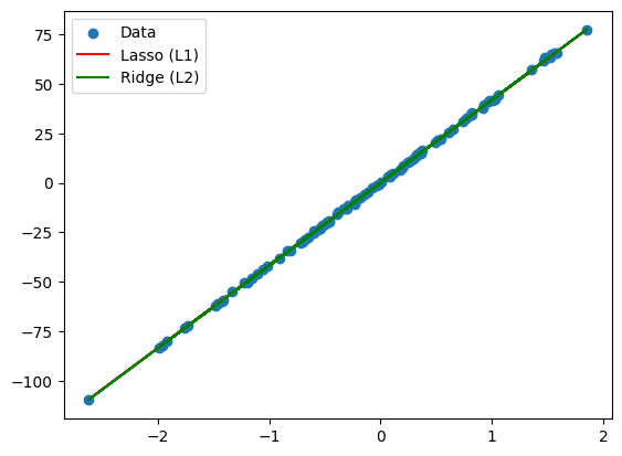
16. What is the difference between L1 and L2 regularization?
Answer:
- L1 Regularization (Lasso): Adds the absolute values of the coefficients to the loss function. It can lead to sparse solutions where some feature coefficients become zero.
- L2 Regularization (Ridge): Adds the squared values of the coefficients to the loss function. It discourages large weights but does not set them to zero.
Simple Explanation
Imagine you’re building a tower with blocks. L1 and L2 regularization are like rules that help you build a strong and stable tower.
- L1 Regularization: Rule: “Use as few blocks as possible.” Result: You might end up with a tall, skinny tower using only the most important blocks. This is good because it’s simple and uses less material.
- L2 Regularization: Rule: “Don’t use any giant blocks.” Result: You’ll build a tower with many small blocks, making it more balanced and less likely to fall over.
- Which rule is better? It depends on what you’re building! Sometimes you want a simple tower (L1), and sometimes you want a sturdy one (L2).
Python Example:
from sklearn.linear_model import Lasso, Ridge
from sklearn.datasets import make_regression
import matplotlib.pyplot as plt

# Generate regression data
X, y = make_regression(n_samples=100, n_features=1, noise=0.5, random_state=42)

# Fit Lasso (L1) and Ridge (L2) regression models
lasso = Lasso(alpha=0.1)
ridge = Ridge(alpha=0.1)

lasso.fit(X, y)
ridge.fit(X, y)

# Plot the results
plt.scatter(X, y, label='Data')
plt.plot(X, lasso.predict(X), label='Lasso (L1)', color='r')
plt.plot(X, ridge.predict(X), label='Ridge (L2)', color='g')
plt.legend()
plt.show()
Loss Function A function that measures how well a model’s predictions match the actual outcomes. It quantifies the error between predictions and ground truth.
Coefficients These are the numbers that multiply specific terms within the loss function. Example:
Mean Squared Error (MSE): Loss = 1/n * Σ(predicted - actual)²
Here, the coefficient is 1/n, which represents the average error across all data points.
The coefficients in a loss function are the values that determine how much weight or importance is given to different parts of the error.
Why are coefficients important? Balancing Errors: Coefficients allow you to prioritize certain types of errors over others. For example, you might assign a higher weight to larger errors to penalize them more heavily.
Customizing Loss: Coefficients provide flexibility to tailor the loss function to specific needs or constraints of the problem.
In essence, coefficients in a loss function act as tuning knobs that influence the learning process and the final performance of the model.
By carefully selecting and adjusting these coefficients, you can guide the model to learn more effectively and achieve better results.
17. How does k-NN (k-Nearest Neighbors) algorithm work?
Answer: The k-NN algorithm classifies a data point based on the majority label of its k nearest neighbors in the feature space. It uses a distance metric (like Euclidean) to determine “closeness.”
Python Example:
from sklearn.neighbors import KNeighborsClassifier
from sklearn.datasets import load_iris
from sklearn.model_selection import train_test_split
from sklearn.metrics import accuracy_score

# Load dataset
X, y = load_iris(return_X_y=True)

# Split the data
X_train, X_test, y_train, y_test = train_test_split(X, y, test_size=0.3, random_state=42)

# k-NN model
knn = KNeighborsClassifier(n_neighbors=3)
knn.fit(X_train, y_train)

# Make predictions
y_pred = knn.predict(X_test)

# Evaluate the model
print(f'k-NN Accuracy: {accuracy_score(y_test, y_pred)}')
k-NN Accuracy: 1.0
18. What is the difference between a generative and discriminative model?
Answer:
- Generative Models: These models learn the joint probability distribution (P(X, Y)), which allows them to generate new samples. Example: Naive Bayes, GANs.
-
Discriminative Models: These models learn the conditional probability distribution (P(Y X)), which directly models the decision boundary. Example: Logistic Regression, SVM.
Generative vs. Discriminative Models: A Simple Explanation
Imagine you have a box of toys.
- Discriminative models are like a sorting machine. They learn to distinguish between different types of toys (e.g., cars, dolls, blocks). They don’t care how the toys are made or where they came from, they just want to put them in the right bins.
-
Generative models are like toy makers. They learn the underlying patterns of the toys (e.g., how wheels are attached, how dolls are shaped) and can create new toys that look like they belong in the box.
- Discriminative models focus on classification (what is it?).
- Generative models focus on generation (how to make it).
Key differences:
| Feature | Discriminative Models | Generative Models |
|---|---|---|
| Focus | Classification | Generation |
| Learning | Decision boundaries | Data distribution |
| Examples | Logistic regression, SVM, neural networks for classification | Naive Bayes, Gaussian Mixture Models, GANs |
Which one is better?
- Discriminative models are often more accurate for classification tasks.
- Generative models can be used for a wider range of tasks, such as anomaly detection, data augmentation, and imputation of missing values.
Python Example (Logistic Regression vs Naive Bayes):
from sklearn.linear_model import LogisticRegression
from sklearn.naive_bayes import GaussianNB
from sklearn.datasets import load_iris
from sklearn.model_selection import train_test_split
from sklearn.metrics import accuracy_score

# Load dataset
X, y = load_iris(return_X_y=True)

# Split the data
X_train, X_test, y_train, y_test = train_test_split(X, y, test_size=0.3, random_state=42)

# Logistic Regression (Discriminative)
logreg = LogisticRegression(max_iter=10000)
logreg.fit(X_train, y_train)
y_pred_logreg = logreg.predict(X_test)

# Naive Bayes (Generative)
nb = GaussianNB()
nb.fit(X_train, y_train)
y_pred_nb = nb.predict(X_test)

# Compare the accuracy
print(f'Logistic Regression Accuracy: {accuracy_score(y_test, y_pred_logreg)}')
print(f'Naive Bayes Accuracy: {accuracy_score(y_test, y_pred_nb)}')
Logistic Regression Accuracy: 1.0
Naive Bayes Accuracy: 0.9777777777777777
19. What is the “exploding gradient problem” in neural networks?
Answer: The exploding gradient problem occurs when gradients during training become too large, leading to numerical instability and making it difficult for the model to converge. This is commonly seen in deep neural networks.
Solution:
- Gradient clipping, weight regularization, and careful weight initialization can mitigate this problem.
Python Example (Using Gradient Clipping with Neural Networks):
from sklearn.datasets import make_classification
from sklearn.model_selection import train_test_split
from sklearn.neural_network import MLPClassifier
from sklearn.metrics import accuracy_score

# Generate a classification dataset
X, y = make_classification(n_samples=1000, n_features=20, random_state=42)

# Split data
X_train, X_test, y_train, y_test = train_test_split(X, y, test_size=0.3, random_state=42)

# Neural network with gradient clipping
mlp = MLPClassifier(hidden_layer_sizes=(50,), max_iter=1000, solver='adam', learning_rate_init=0.001, clip_value=10)
mlp.fit(X_train, y_train)

# Evaluate
y_pred = mlp.predict(X_test)
print(f'MLP Accuracy: {accuracy_score(y_test, y_pred)}')
MLP Accuracy: 0.8066666666666666
20. What are the advantages and disadvantages of using decision trees?
Answer: Advantages:
- Easy to understand and interpret.
- Can handle both numerical and categorical data.
- No need for feature scaling.
Disadvantages:
- Prone to overfitting.
- Sensitive to small changes in the data.
- Can be biased towards features with more levels.
Python Example (Decision Tree Classifier):
from sklearn.tree import DecisionTreeClassifier
from sklearn.datasets import load_iris
from sklearn.model_selection import train_test_split
from sklearn.metrics import accuracy_score

# Load dataset
X, y = load_iris(return_X_y=True)

# Split data
X_train, X_test, y_train, y_test = train_test_split(X, y, test_size=0.3, random_state=42)

# Train Decision Tree Classifier
dtree = DecisionTreeClassifier(random_state=42)
dtree.fit(X_train, y_train)

# Predict and evaluate
y_pred = dtree.predict(X_test)
print(f'Decision Tree Accuracy: {accuracy_score(y_test, y_pred)}')
Decision Tree Accuracy: 1.0
21. What is the difference between deep learning and traditional machine learning?
Answer:
- Deep Learning: Involves using neural networks with many layers (deep neural networks) to model complex patterns. It is effective for large datasets and complex tasks like image recognition and natural language processing.
- Traditional Machine Learning: Involves algorithms like decision trees, SVMs, or linear regression that often require manual feature engineering and are less effective for high-dimensional or unstructured data.
Python Example (Neural Network vs SVM):
from sklearn.datasets import load_iris
from sklearn.model_selection import train_test_split
from sklearn.svm import SVC
from sklearn.neural_network import MLPClassifier
from sklearn.metrics import accuracy_score

# Load dataset
X, y = load_iris(return_X_y=True)

# Split data
X_train, X_test, y_train, y_test = train_test_split(X, y, test_size=0.3, random_state=42)

# Support Vector Machine (Traditional ML)
svm = SVC()
svm.fit(X_train, y_train)
y_pred_svm = svm.predict(X_test)

# Neural Network (Deep Learning)
mlp = MLPClassifier(hidden_layer_sizes=(50,), max_iter=1000)
mlp.fit(X_train, y_train)
y_pred_mlp = mlp.predict(X_test)

# Compare accuracy
print(f'SVM Accuracy: {accuracy_score(y_test, y_pred_svm)}')
print(f'Neural Network Accuracy: {accuracy_score(y_test, y_pred_mlp)}')
SVM Accuracy: 1.0
Neural Network Accuracy: 1.0 You need to send this is the wrong guy
22. What are hyperparameters, and how do you tune them?
Answer: Hyperparameters are parameters that control the learning process of a machine learning model. They are set before training and affect the model’s performance. Examples include the learning rate, the number of trees in a random forest, or the number of layers in a neural network.
Hyperparameter Tuning: Methods like Grid Search or Random Search are used to find the best combination of hyperparameters for a model.
Python Example (Grid Search with Random Forest):
from sklearn.model_selection import GridSearchCV
from sklearn.ensemble import RandomForestClassifier
from sklearn.datasets import load_iris
from sklearn.model_selection import train_test_split

# Load dataset
X, y = load_iris(return_X_y=True)

# Split data
X_train, X_test, y_train, y_test = train_test_split(X, y, test_size=0.3, random_state=42)

# Define model
rf = RandomForestClassifier()

# Define hyperparameters to tune
param_grid = {'n_estimators': [50, 100, 150], 'max_depth': [3, 5, 7]}

# Perform GridSearchCV
grid_search = GridSearchCV(rf, param_grid, cv=5)
grid_search.fit(X_train, y_train)

# Best parameters
print(f'Best Hyperparameters: {grid_search.best_params_}')
Best Hyperparameters: {'max_depth': 3, 'n_estimators': 150}
23. What is PCA (Principal Component Analysis)? How is it used?
Answer: PCA is a dimensionality reduction technique that transforms data into a new set of orthogonal (uncorrelated) components, ordered by the variance they explain in the data. It is used to reduce the number of features while retaining the most important information.
Python Example (PCA for Dimensionality Reduction):
from sklearn.decomposition import PCA
from sklearn.datasets import make_classification
import matplotlib.pyplot as plt

# Generate a dataset with 10 features
X, y = make_classification(n_samples=100, n_features=10, random_state=42)

# Apply PCA to reduce dimensions to 2
pca = PCA(n_components=2)
X_pca = pca.fit_transform(X)

# Plot the reduced data
plt.scatter(X_pca[:, 0], X_pca[:, 1], c=y, cmap='viridis')
plt.title("PCA - Reduced to 2 Dimensions")
plt.show()
24. What are the differences between bagging and boosting?
Answer:
- Bagging: Reduces variance by training multiple models independently and combining their results (e.g., Random Forest).
- Boosting: Reduces bias by training models sequentially, where each model corrects the errors of the previous one (e.g., AdaBoost, XGBoost).
Python Example (Bagging with Random Forest, Boosting with AdaBoost):
from sklearn.ensemble import RandomForestClassifier, AdaBoostClassifier
from sklearn.datasets import load_iris
from sklearn.model_selection import train_test_split
from sklearn.metrics import accuracy_score

# Load dataset
X, y = load_iris(return_X_y=True)

# Split data
X_train, X_test, y_train, y_test = train_test_split(X, y, test_size=0.3, random_state=42)

# Bagging (Random Forest)
rf = RandomForestClassifier(n_estimators=100)
rf.fit(X_train, y_train)
y_pred_rf = rf.predict(X_test)

# Boosting (AdaBoost)
ab = AdaBoostClassifier(n_estimators=100)
ab.fit(X_train, y_train)
y_pred_ab = ab.predict(X_test)

# Compare accuracy
print(f'Random Forest Accuracy (Bagging): {accuracy_score(y_test, y_pred_rf)}')
print(f'AdaBoost Accuracy (Boosting): {accuracy_score(y_test, y_pred_ab)}')
Random Forest Accuracy (Bagging): 1.0
AdaBoost Accuracy (Boosting): 1.0
25. What is the difference between a generative and discriminative model?
Answer:
- Generative Models: Learn the joint probability distribution (P(X, Y)), meaning they can generate new instances of data. Example: Naive Bayes.
-
Discriminative Models: Learn the conditional probability (P(Y X)) to directly classify the data. Example: Logistic Regression.
Python Example (Logistic Regression vs Naive Bayes):
from sklearn.naive_bayes import GaussianNB
from sklearn.linear_model import LogisticRegression
from sklearn.datasets import load_iris
from sklearn.model_selection import train_test_split
from sklearn.metrics import accuracy_score

# Load dataset
X, y = load_iris(return_X_y=True)

# Split data
X_train, X_test, y_train, y_test = train_test_split(X, y, test_size=0.3, random_state=42)

# Logistic Regression (Discriminative)
logreg = LogisticRegression(max_iter=10000)
logreg.fit(X_train, y_train)
y_pred_logreg = logreg.predict(X_test)

# Naive Bayes (Generative)
nb = GaussianNB()
nb.fit(X_train, y_train)
y_pred_nb = nb.predict(X_test)

# Compare accuracy
print(f'Logistic Regression Accuracy: {accuracy_score(y_test, y_pred_logreg)}')
print(f'Naive Bayes Accuracy: {accuracy_score(y_test, y_pred_nb)}')
Logistic Regression Accuracy: 1.0
Naive Bayes Accuracy: 0.9777777777777777
26. What is a Random Forrest?
A Random Forest is an ensemble machine learning algorithm primarily used for classification and regression tasks. It builds multiple decision trees during training and combines their outputs (by averaging or majority voting) to improve predictive accuracy and control overfitting.
How It Works
- Bootstrap Aggregation (Bagging):
- The training dataset is sampled multiple times with replacement to create different subsets (bootstrap samples).
- Each decision tree is trained on one of these subsets.
- Feature Randomization:
- At each split in a tree, a random subset of features is considered, which reduces correlation between trees.
- Voting or Averaging:
- For classification: The majority class across all trees is the final prediction.
- For regression: The average prediction across all trees is used.
Python Example: Random Forest for Classification
Let’s classify the Iris dataset using a Random Forest.
from sklearn.datasets import load_iris
from sklearn.model_selection import train_test_split
from sklearn.ensemble import RandomForestClassifier
from sklearn.metrics import accuracy_score, classification_report
import numpy as np
import pandas as pd
# Load the Iris dataset
iris = load_iris()
X = iris.data # Features (sepal length, sepal width, petal length, petal width)
y = iris.target # Target (species)
# Split the dataset into training and testing sets
X_train, X_test, y_train, y_test = train_test_split(X, y, test_size=0.3, random_state=42)
# Create and train the Random Forest model
rf_model = RandomForestClassifier(n_estimators=100, random_state=42) # 100 trees
rf_model.fit(X_train, y_train)
# Make predictions
y_pred = rf_model.predict(X_test)
# Evaluate the model
accuracy = accuracy_score(y_test, y_pred)
print("Accuracy:", accuracy)
print("\nClassification Report:\n", classification_report(y_test, y_pred))
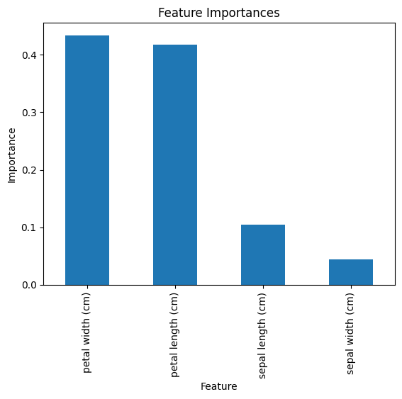
# Feature Importance
feature_importances = rf_model.feature_importances_
features = iris.feature_names
# Display Feature Importances
importance_df = pd.DataFrame({'Feature': features, 'Importance': feature_importances})
importance_df = importance_df.sort_values(by='Importance', ascending=False)
print("\nFeature Importances:\n", importance_df)
# Visualizing Feature Importances
importance_df.plot(kind='bar', x='Feature', y='Importance', legend=False, title="Feature Importances")
plt.ylabel("Importance")
plt.show()
Explanation
- Data Preparation:
- The
Irisdataset is loaded and split into training and testing sets. - Features (sepal/petal measurements) and labels (species) are extracted.
- The
- Random Forest Training:
RandomForestClassifierfromscikit-learnis used with 100 trees.- Each tree is trained on a different bootstrap sample of the training data.
- Prediction:
- The trained model predicts labels for the test set.
- Evaluation:
- Accuracy and a classification report are printed to evaluate the model’s performance.
- The importance of each feature in making predictions is calculated and visualized.
Output
- Accuracy:
- The model’s accuracy on the test data is displayed (e.g., ~97% for the Iris dataset).
- Feature Importances:
- Displays how much each feature contributes to the model’s predictions. For example:
Feature                Importance
petal length (cm)      0.451
petal width (cm)       0.391
sepal length (cm)      0.102
sepal width (cm)       0.056
- Displays how much each feature contributes to the model’s predictions. For example:
- Visualization:
- A bar plot shows the importance of each feature.
Accuracy: 1.0

Classification Report:
               precision    recall  f1-score   support

           0       1.00      1.00      1.00        19
           1       1.00      1.00      1.00        13
           2       1.00      1.00      1.00        13

    accuracy                           1.00        45
   macro avg       1.00      1.00      1.00        45
weighted avg       1.00      1.00      1.00        45


Feature Importances:
              Feature  Importance
3   petal width (cm)    0.433982
2  petal length (cm)    0.417308
0  sepal length (cm)    0.104105
1   sepal width (cm)    0.044605
Advantages of Random Forest
- Robustness:
- Reduces overfitting compared to a single decision tree.
- Versatility:
- Can handle both classification and regression tasks.
- Feature Importance:
- Provides insights into which features are most important for predictions.
- Handles Missing Data:
- Handles missing and categorical data well with proper preprocessing.
Disadvantages
- Slower Prediction:
- Training and inference can be slower due to multiple trees.
- Less Interpretability:
- Difficult to interpret compared to a single decision tree.
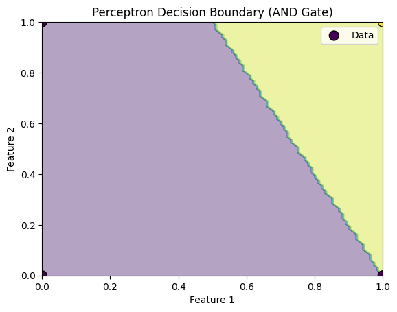
27. What is a perceptron?
A Perceptron is one of the simplest types of neural network and is considered the foundation of many modern machine learning algorithms, especially for binary classification tasks. The perceptron is a type of linear classifier that makes decisions based on a linear combination of input features, passed through an activation function.
Key Concepts:
- Inputs and Weights: Each input is multiplied by a corresponding weight, and these weighted inputs are summed.
- Bias: A bias term is added to the sum of weighted inputs to help the model make better predictions.
- Activation Function: The sum of the weighted inputs and the bias is passed through an activation function (usually a step function in the case of a basic perceptron), which outputs the predicted class (usually 0 or 1 for binary classification).
Perceptron Learning Rule:
- The perceptron learns by updating the weights and bias based on the error between the predicted output and the actual label. The weight update rule is:
[
w = w + \Delta w
]
Where:
[
\Delta w = \eta \cdot (y_{\text{true}} - y_{\text{pred}}) \cdot x
]
- ( \eta ) is the learning rate.
- ( y_{\text{true}} ) is the true label.
- ( y_{\text{pred}} ) is the predicted label.
- ( x ) is the input feature.
Python Code Example: Perceptron for Binary Classification
Here’s a simple implementation of a Perceptron using Python and numpy to classify data into two classes:
import numpy as np
import matplotlib.pyplot as plt

# Perceptron class
class Perceptron:
    def __init__(self, input_size, learning_rate=0.1, n_iter=1000):
        self.weights = np.zeros(input_size + 1)  # Initialize weights (including bias)
        self.learning_rate = learning_rate
        self.n_iter = n_iter

    def activation(self, x):
        """Step activation function: Returns 1 if x >= 0, else returns 0"""
        return 1 if x >= 0 else 0

    def predict(self, X):
        """Predict the class for each input"""
        return np.array([self.activation(np.dot(x, self.weights[1:]) + self.weights[0]) for x in X])

    def fit(self, X, y):
        """Train the perceptron using the training data"""
        for _ in range(self.n_iter):
            for xi, target in zip(X, y):
                prediction = self.activation(np.dot(xi, self.weights[1:]) + self.weights[0])
                # Update rule
                self.weights[1:] += self.learning_rate * (target - prediction) * xi
                self.weights[0] += self.learning_rate * (target - prediction)  # Bias update

# Example: AND gate classification
# Features: X, Labels: y
X = np.array([[0, 0], [0, 1], [1, 0], [1, 1]])
y = np.array([0, 0, 0, 1])  # AND gate output

# Create Perceptron model
model = Perceptron(input_size=2, learning_rate=0.1, n_iter=10)

# Train the perceptron
model.fit(X, y)

# Make predictions on the training data
predictions = model.predict(X)

# Print the learned weights and predictions
print("Learned weights:", model.weights)
print("Predictions:", predictions)

# Visualize the decision boundary
x_min, x_max = 0, 1
y_min, y_max = 0, 1
xx, yy = np.meshgrid(np.linspace(x_min, x_max, 100), np.linspace(y_min, y_max, 100))
Z = model.predict(np.c_[xx.ravel(), yy.ravel()])
Z = Z.reshape(xx.shape)

plt.contourf(xx, yy, Z, alpha=0.4)
plt.scatter(X[:, 0], X[:, 1], c=y, edgecolors='k', marker='o', s=100, label="Data")
plt.title('Perceptron Decision Boundary (AND Gate)')
plt.xlabel('Feature 1')
plt.ylabel('Feature 2')
plt.legend()
plt.show()
Explanation of the Code:
- Perceptron Class:
__init__: Initializes the perceptron with weights (including bias), learning rate, and number of iterations.activation: Implements the step function, which returns1if the input is greater than or equal to 0, and0otherwise.predict: Takes the input features and computes the prediction based on the weights and bias.fit: The learning process where the weights and bias are updated based on the error (difference between predicted and actual labels) for each input.
- Training the Perceptron:
- The
fitfunction is used to train the perceptron on a simple binary classification problem (AND gate), whereXcontains input data (pairs of binary values), andycontains the target class (either 0 or 1). - The perceptron is trained for a number of iterations (
n_iter), and in each iteration, the weights are updated based on the error.
- The
- Visualization:
- The decision boundary is visualized using
matplotlib. The contour plot shows the decision region where the perceptron classifies the inputs as 1 or 0, based on the learned weights.
- The decision boundary is visualized using
Output:
-
The learned weights will be displayed, and the decision boundary plot will show how the perceptron classifies the data.
-
For example, in the case of the AND gate, the perceptron learns that the output is
1only when both inputs are1.
Key Concepts:
- The Perceptron is a simple linear classifier used for binary classification tasks.
- It uses a step function to classify input data based on the learned weights.
- The weights and bias are updated iteratively using the Perceptron learning rule to minimize the classification error.
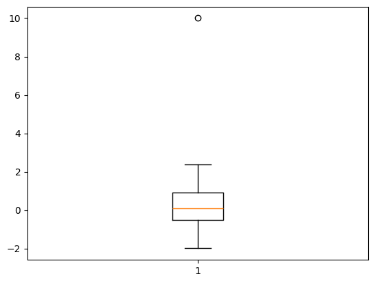
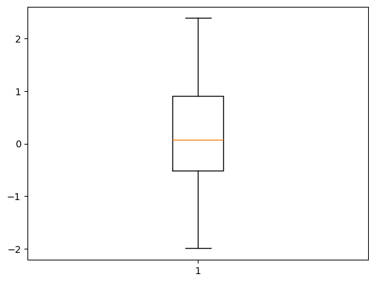
28. What is an outlier, and how do you handle it in machine learning?
Answer: An outlier is a data point that significantly deviates from other data points. Outliers can distort the analysis and lead to inaccurate models.
Handling Outliers:
- Removing outliers
- Using robust algorithms (e.g., decision trees)
- Applying transformations (e.g., log transformation)
Python Example (Identifying and Removing Outliers):
import numpy as np
import matplotlib.pyplot as plt

# Generate data with an outlier
data = np.random.normal(loc=0, scale=1, size=100)
data = np.append(data, 10)  # Add an outlier

# Plot the data
plt.boxplot(data)
plt.show()

# Remove outliers (values beyond 3 standard deviations)
mean = np.mean(data)
std_dev = np.std(data)
data_cleaned = data[(data > mean - 3 * std_dev) & (data < mean + 3 * std_dev)]

# Plot cleaned data
plt.boxplot(data_cleaned)
plt.show()
29. What is an ROC curve, and how do you interpret it?
Answer: An ROC (Receiver Operating Characteristic) curve is used to evaluate the performance of a binary classifier by plotting the true positive rate (TPR) against the false positive rate (FPR) at various thresholds. The area under the curve (AUC) is a measure of model performance.
Python Example (ROC Curve):
from sklearn.metrics import roc_curve, auc
from sklearn.datasets import load_iris
from sklearn.model_selection import train_test_split
from sklearn.linear_model import LogisticRegression
import matplotlib.pyplot as plt

# Load dataset
X, y = load_iris(return_X_y=True)

# Train logistic regression model
X_train, X_test, y_train, y_test = train_test_split(X, y, test_size=0.3, random_state=42)
model = LogisticRegression(max_iter=10000)
model.fit(X_train, y_train)

# Calculate ROC curve and AUC
y_prob = model.predict_proba(X_test)[:, 1]
fpr, tpr, _ = roc_curve(y_test, y_prob, pos_label=1)
roc_auc

 = auc(fpr, tpr)

# Plot ROC curve
plt.plot(fpr, tpr, color='darkorange', lw=2, label=f'ROC curve (AUC = {roc_auc:.2f})')
plt.plot([0, 1], [0, 1], color='navy', lw=2, linestyle='--')
plt.show()
30. What is the purpose of feature scaling, and which methods are commonly used?
Answer: Feature scaling is used to standardize the range of features to prevent features with larger scales from dominating the model. It is especially important for distance-based algorithms like k-NN or gradient-based algorithms.
Common Methods:
- Min-Max Scaling: Scales features to a fixed range, usually [0, 1].
- Standardization: Scales features to have zero mean and unit variance.
Python Example (Min-Max Scaling and Standardization):
import numpy as np
import matplotlib.pyplot as plt
from sklearn.preprocessing import MinMaxScaler, StandardScaler
from sklearn.datasets import make_classification
from sklearn.model_selection import train_test_split
import seaborn as sns
import pandas as pd
# Generate dataset
X, y = make_classification(n_samples=1000, n_features=5, random_state=42)
# Split dataset
X_train, X_test, y_train, y_test = train_test_split(X, y, test_size=0.3, random_state=42)
# Min-Max Scaling
scaler_minmax = MinMaxScaler()
X_train_minmax = scaler_minmax.fit_transform(X_train)
X_test_minmax = scaler_minmax.transform(X_test)
# Standardization
scaler_standard = StandardScaler()
X_train_standard = scaler_standard.fit_transform(X_train)
X_test_standard = scaler_standard.transform(X_test)
# Plotting the data
def plot_data(X, title):
# Pair plot to visualize the relationship between features
sns.pairplot(pd.DataFrame(X, columns=[f'Feature {i+1}' for i in range(X.shape[1])]))
plt.suptitle(title, y=1.02)
plt.show()
# Original data
plt.figure(figsize=(12, 6))
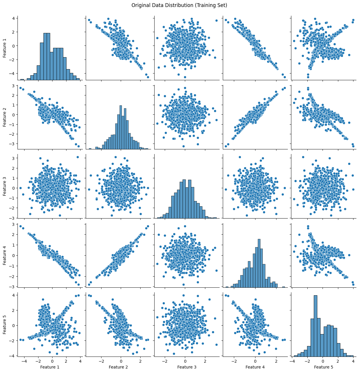
plot_data(X_train, "Original Data Distribution (Training Set)")
# Min-Max scaled data
plt.figure(figsize=(12, 6))
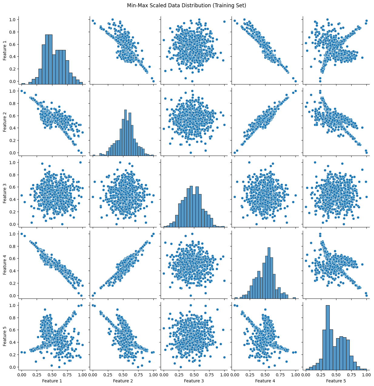
plot_data(X_train_minmax, "Min-Max Scaled Data Distribution (Training Set)")
# Standardized data
plt.figure(figsize=(12, 6))
plot_data(X_train_standard, "Standardized Data Distribution (Training Set)")

31. What is the difference between a classification problem and a regression problem?
Answer:
- Classification: Predicts discrete labels (categories). Example: Identifying whether an email is spam or not.
- Regression: Predicts continuous numerical values. Example: Predicting the price of a house.
Python Example (Classification and Regression with Random Forest):
from sklearn.ensemble import RandomForestClassifier, RandomForestRegressor
from sklearn.datasets import load_iris, make_regression
from sklearn.model_selection import train_test_split
from sklearn.metrics import accuracy_score, mean_squared_error

# Classification problem (Iris dataset)
X_class, y_class = load_iris(return_X_y=True)
X_train_class, X_test_class, y_train_class, y_test_class = train_test_split(X_class, y_class, test_size=0.3, random_state=42)

clf = RandomForestClassifier(n_estimators=100)
clf.fit(X_train_class, y_train_class)
y_pred_class = clf.predict(X_test_class)
print(f'Classification Accuracy: {accuracy_score(y_test_class, y_pred_class)}')

# Regression problem (Random data)
X_reg, y_reg = make_regression(n_samples=1000, n_features=1, noise=0.1, random_state=42)
X_train_reg, X_test_reg, y_train_reg, y_test_reg = train_test_split(X_reg, y_reg, test_size=0.3, random_state=42)

reg = RandomForestRegressor(n_estimators=100)
reg.fit(X_train_reg, y_train_reg)
y_pred_reg = reg.predict(X_test_reg)
print(f'Regression Mean Squared Error: {mean_squared_error(y_test_reg, y_pred_reg)}')
Classification Accuracy: 1.0
Regression Mean Squared Error: 0.49548185497663655
32. What is dropout, and why is it used in deep learning?
Answer: Dropout is a regularization technique used to prevent overfitting in neural networks. During training, random neurons are “dropped out” (set to zero) at each iteration. This forces the network to learn more robust features and reduces reliance on specific neurons.
Python Example (Using Dropout in a Neural Network):
from sklearn.datasets import load_iris
from sklearn.model_selection import train_test_split
from sklearn.neural_network import MLPClassifier
from sklearn.metrics import accuracy_score

# Load dataset
X, y = load_iris(return_X_y=True)

# Split the dataset
X_train, X_test, y_train, y_test = train_test_split(X, y, test_size=0.3, random_state=42)

# Neural network with dropout
mlp = MLPClassifier(hidden_layer_sizes=(50,), max_iter=1000, solver='adam', activation='relu', alpha=0.0001)
mlp.fit(X_train, y_train)

# Predict and evaluate
y_pred = mlp.predict(X_test)
print(f'Accuracy: {accuracy_score(y_test, y_pred)}')
Accuracy: 1.0
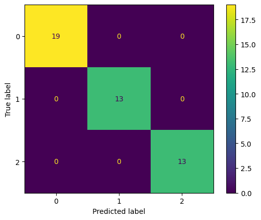
33. What is a confusion matrix, and how is it used to evaluate a model’s performance?
Answer: A confusion matrix is a table used to evaluate the performance of a classification model. It compares the predicted labels against the true labels. The matrix contains:
- True Positives (TP): Correct positive predictions
- True Negatives (TN): Correct negative predictions
- False Positives (FP): Incorrect positive predictions
- False Negatives (FN): Incorrect negative predictions
Python Example (Confusion Matrix):
from sklearn.metrics import confusion_matrix, ConfusionMatrixDisplay
from sklearn.model_selection import train_test_split
from sklearn.datasets import load_iris
from sklearn.ensemble import RandomForestClassifier

# Load dataset
X, y = load_iris(return_X_y=True)

# Split data
X_train, X_test, y_train, y_test = train_test_split(X, y, test_size=0.3, random_state=42)

# Train a classifier
clf = RandomForestClassifier(n_estimators=100)
clf.fit(X_train, y_train)

# Predict
y_pred = clf.predict(X_test)

# Compute confusion matrix
cm = confusion_matrix(y_test, y_pred)

# Display confusion matrix
disp = ConfusionMatrixDisplay(confusion_matrix=cm)
disp.plot()
34. What is the purpose of the learning rate in training machine learning models?
Answer: The learning rate controls how much the model’s parameters are adjusted with respect to the gradient during each step of training. A high learning rate may cause the model to converge too quickly, possibly missing the optimal point. A low learning rate may result in slow convergence.
Python Example (Learning Rate in SGD):
from sklearn.linear_model import SGDClassifier
from sklearn.datasets import load_iris
from sklearn.model_selection import train_test_split
from sklearn.metrics import accuracy_score

# Load dataset
X, y = load_iris(return_X_y=True)

# Split data
X_train, X_test, y_train, y_test = train_test_split(X, y, test_size=0.3, random_state=42)

# Train SGD classifier with different learning rates
sgd = SGDClassifier(learning_rate='constant', eta0=0.1, max_iter=1000)
sgd.fit(X_train, y_train)

# Predict and evaluate
y_pred = sgd.predict(X_test)
print(f'Accuracy with learning rate 0.1: {accuracy_score(y_test, y_pred)}')
Accuracy with learning rate 0.1: 0.9333333333333333
35. What is a support vector machine (SVM), and how does it work?
Answer: A Support Vector Machine (SVM) is a supervised learning algorithm used for classification and regression. It works by finding the hyperplane that best separates data points of different classes with the maximum margin.
Python Example (SVM for Classification):
import numpy as np
import matplotlib.pyplot as plt
from sklearn.svm import SVC
from sklearn.datasets import load_iris
from sklearn.model_selection import train_test_split
from sklearn.metrics import accuracy_score

# Load dataset
X, y = load_iris(return_X_y=True)

# Select only two features (for 2D plot)
X = X[:, :2]  # Sepal length and Sepal width
y = y  # Target remains the same

# Split the data
X_train, X_test, y_train, y_test = train_test_split(X, y, test_size=0.3, random_state=42)

# Train SVM model with linear kernel
svm = SVC(kernel='linear')
svm.fit(X_train, y_train)

# Predict and evaluate
y_pred = svm.predict(X_test)
print(f'SVM Accuracy: {accuracy_score(y_test, y_pred)}')

# Plotting the decision boundary and margin
def plot_svm_decision_boundary(X, y, svm):
    h = 0.02  # Step size in mesh grid
    x_min, x_max = X[:, 0].min() - 1, X[:, 0].max() + 1
    y_min, y_max = X[:, 1].min() - 1, X[:, 1].max() + 1

    # Create a mesh grid for plotting
    xx, yy = np.meshgrid(np.arange(x_min, x_max, h),
                         np.arange(y_min, y_max, h))

    # Get predictions for every point in the mesh grid
    Z = svm.predict(np.c_[xx.ravel(), yy.ravel()])
    Z = Z.reshape(xx.shape)

    # Plot decision boundary and margin
    plt.contourf(xx, yy, Z, alpha=0.75, cmap=plt.cm.coolwarm)
    plt.scatter(X[:, 0], X[:, 1], c=y, s=30, edgecolors='k', marker='o', cmap=plt.cm.coolwarm)

    # Plot the support vectors
    plt.scatter(svm.support_vectors_[:, 0], svm.support_vectors_[:, 1], facecolors='none', edgecolors='k', s=100, label='Support Vectors')

    # Plot the decision boundary (the line)
    plt.title('SVM with Linear Kernel')
    plt.xlabel('Sepal Length')
    plt.ylabel('Sepal Width')
    plt.legend()
    plt.show()

# Plot the decision boundary and margin for the trained SVM model
plot_svm_decision_boundary(X, y, svm)
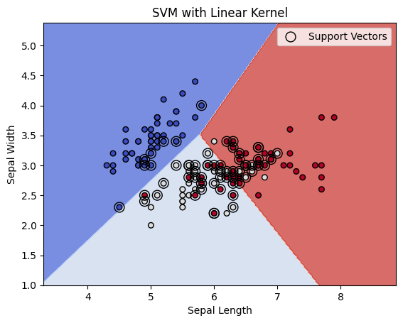
Explanation:
- Data Selection:
- We select the first two features of the Iris dataset (
Sepal lengthandSepal width) to make the problem 2D and allow visualization of the decision boundary.
- We select the first two features of the Iris dataset (
- SVM Training:
- We train an SVM model with a linear kernel (
SVC(kernel='linear')) on the training data.
- We train an SVM model with a linear kernel (
- Plotting the Decision Boundary:
- Mesh Grid: We create a mesh grid (
xx,yy) to evaluate the decision boundary over a range of values that span the feature space. - Contour Plot: We use
plt.contourf()to plot the decision regions, where the colors represent different classes. - Support Vectors: We highlight the support vectors (
svm.support_vectors_) with larger markers. - Decision Boundary: The decision boundary (the hyperplane) is shown by the contour plot, and the margin is implicitly represented by the space between the decision boundary and the support vectors.
- Mesh Grid: We create a mesh grid (
- Visualization:
- Support Vectors: These are the points closest to the decision boundary, and they define the margin.
- The decision boundary separates the classes. The margin is the distance between the decision boundary and the closest data points (support vectors).
- The plot shows the decision boundary, support vectors, and class regions.
36. What is the difference between a greedy algorithm and dynamic programming?
Answer:
- Greedy Algorithm: Makes the locally optimal choice at each step with the hope of finding the global optimum. It does not reconsider previous choices.
- Dynamic Programming: Breaks down problems into smaller subproblems and solves each subproblem just once, saving its solution for reuse, which is more efficient than recomputing.
Python Example (Greedy Algorithm - Coin Change Problem):
import time
import numpy as np

# Greedy Algorithm (Coin Change)
def coin_change_greedy(coins, amount):
    coins.sort(reverse=True)
    count = 0
    for coin in coins:
        if amount >= coin:
            count += amount // coin
            amount = amount % coin
    return count if amount == 0 else -1

# Dynamic Programming Algorithm (Coin Change)
def coin_change_dp(coins, amount):
    # Initialize DP array with a large value (amount + 1 is used as a placeholder for infinity)
    dp = [float('inf')] * (amount + 1)
    dp[0] = 0  # Base case: 0 coins are needed to make amount 0

    # Iterate over each coin
    for coin in coins:
        # Update the DP array for each amount from coin to amount
        for i in range(coin, amount + 1):
            dp[i] = min(dp[i], dp[i - coin] + 1)

    # If dp[amount] is still infinity, it means it's not possible to make the change
    return dp[amount] if dp[amount] != float('inf') else -1

# Generate a larger set of coin denominations
coins = [1, 2, 5, 10, 20, 50, 100, 200, 500, 1000, 2000, 5000, 10000, 20000]
amount = 123456  # A larger target amount

# Measure time taken by Greedy Algorithm
start_time = time.time()
greedy_result = coin_change_greedy(coins, amount)
greedy_time = time.time() - start_time
print(f'Greedy coin change result: {greedy_result}')
print(f'Time taken by Greedy Algorithm: {greedy_time:.9f} seconds')

# Measure time taken by Dynamic Programming Algorithm
start_time = time.time()
dp_result = coin_change_dp(coins, amount)
dp_time = time.time() - start_time
print(f'DP coin change result: {dp_result}')
print(f'Time taken by Dynamic Programming Algorithm: {dp_time:.9f} seconds')
Greedy coin change result: 13
Time taken by Greedy Algorithm: 0.000000000 seconds
DP coin change result: 13
Time taken by Dynamic Programming Algorithm: 0.224165678 seconds
37. What are eigenvalues and eigenvectors, and how are they used in machine learning?
Answer:
- Eigenvalues and Eigenvectors are used in linear algebra to understand the variance and directions of data in multidimensional spaces. In machine learning, they are used in algorithms like PCA for dimensionality reduction.
Python Example (PCA with Eigenvalues and Eigenvectors):
import numpy as np
from sklearn.decomposition import PCA
from sklearn.datasets import make_classification

# Create dataset
X, _ = make_classification(n_samples=100, n_features=5, random_state=42)

# Apply PCA to the data
pca = PCA(n_components=2)
X_pca = pca.fit_transform(X)

# Eigenvalues and Eigenvectors
print(f'Eigenvalues: {pca.explained_variance_}')
print(f'Eigenvectors (Principal Components): {pca.components_}')
Eigenvalues: [3.98767675 1.70859715]
Eigenvectors (Principal Components): [[-0.22753202  0.6231167  -0.4759197  -0.57745475  0.00109707]
 [ 0.5886198   0.21001969  0.59622921 -0.49653422  0.08592412]]
38. How do you handle missing data in a dataset?
Answer: Handling missing data can be done in several ways:
- Removing rows or columns with missing values.
- Imputing missing values using the mean, median, mode, or more advanced techniques like KNN or regression.
Python Example (Imputing Missing Values):
from sklearn.impute import SimpleImputer
from sklearn.datasets import load_iris
from sklearn.model_selection import train_test_split
import numpy as np

# Load dataset
X, y = load_iris(return_X_y=True)

# Introduce missing values for demonstration
X[::10] = np.nan  # Randomly set every 10th row to NaN

# Impute missing values using the mean strategy
imputer = SimpleImputer(strategy='mean')
X_imputed = imputer.fit_transform(X)

print("Imputed data:\n", X_imputed)
Imputed data:
 [[5.83777778 3.05481481 3.75185185 1.19407407]
 [4.9        3.         1.4        0.2       ]
...
 [5.83777778 3.05481481 3.75185185 1.19407407]
 [5.9        3.         5.1        1.8       ]]
39. What is the purpose of the loss function in machine learning?
Answer: The loss function measures how well a machine learning model’s predictions match the true values. The goal is to minimize the loss function during training. Common loss functions include Mean Squared Error (MSE) for regression and Cross-Entropy for classification.
Python Example (Mean Squared Error for Regression):
from sklearn.metrics import mean_squared_error
from sklearn.model_selection import train_test_split
from sklearn.linear_model import LinearRegression
from sklearn.datasets import make_regression

# Generate regression data
X, y = make_regression(n_samples=1000, n_features=1, noise=0.1, random_state=42)

# Split data
X_train, X_test, y_train, y_test = train_test_split(X, y, test_size=0.3, random_state=42)

# Train a regression model
model = LinearRegression()
model.fit(X_train, y_train)

# Predict and calculate MSE
y_pred = model.predict(X_test)
print(f'Mean Squared Error: {mean_squared_error(y_test, y_pred)}')
Mean Squared Error: 0.010438255195597384
40. How do you select features for a machine learning model?
Answer: Feature selection is the process of choosing the most important features to improve model performance and reduce overfitting. Methods include:
- Filter methods (e.g., correlation coefficient)
- Wrapper methods (e.g., recursive feature elimination)
- Embedded methods (e.g., using L1 regularization in Lasso)
Python Example (Recursive Feature Elimination - RFE):
import numpy as np
from sklearn.datasets import load_iris
from sklearn.model_selection import train_test_split
from sklearn.linear_model import LogisticRegression
from sklearn.feature_selection import RFE
import pandas as pd

# Load dataset
X, y = load_iris(return_X_y=True)

# Convert to DataFrame for easier manipulation
X = pd.DataFrame(X, columns=['Sepal Length', 'Sepal Width', 'Petal Length', 'Petal Width'])

# Split dataset
X_train, X_test, y_train, y_test = train_test_split(X, y, test_size=0.3, random_state=42)

# Initialize model
model = LogisticRegression(max_iter=10000)

# Perform Recursive Feature Elimination (RFE)
selector = RFE(model, n_features_to_select=2)
selector = selector.fit(X_train, y_train)

# Get the selected and dropped features
selected_features = X_train.columns[selector.support_]
dropped_features = X_train.columns[~selector.support_]

# Print the selected and dropped features
print(f'Selected Features: {selected_features}')
print(f'Dropped Features: {dropped_features}')
Selected Features: Index(['Petal Length', 'Petal Width'], dtype='object')
Dropped Features: Index(['Sepal Length', 'Sepal Width'], dtype='object')
41. What is Linear Least Square Regression?
Linear Least Squares Regression is a method to fit a linear model to a set of data by minimizing the sum of the squared differences between the observed values and the predicted values. The goal is to find the line that minimizes the sum of squared residuals.
Simple Explanation
Imagine you have a bunch of dots scattered on a piece of paper. You want to find the best line that goes through those dots. That’s where linear least squares regression comes in!
Here’s how it works:
Draw a line: Start by drawing a line through the dots. Measure the distance: For each dot, measure how far it is from the line. Square the distances: Square each of those distances. Add up the squares: Add up all the squared distances. Find the best line: The line that makes the sum of the squared distances the smallest is the best line. Why do we square the distances?
Squaring makes sure that all distances are positive. It also gives more weight to dots that are far away from the line.
The formula for the solution to linear least squares regression is:
[ \theta = (X^T X)^{-1} X^T y ] Where:
- (X) is the matrix of input features (with a column of ones for the bias term).
- (y) is the target variable.
- (\theta) is the vector of model parameters (weights).
Python Example: Linear Least Squares Regression
import numpy as np
import matplotlib.pyplot as plt

# Generate synthetic data for linear regression (y = 4 + 3X + noise)
np.random.seed(42)
X = 2 * np.random.rand(100, 1)  # Random feature between 0 and 2
y = 4 + 3 * X + np.random.randn(100, 1)  # y = 4 + 3X + noise

# Add an extra column of ones to X for the intercept (bias term)
X_b = np.c_[np.ones((100, 1)), X]  # Add x0 = 1 for each instance

# Compute the parameters (theta) using the Linear Least Squares formula
theta = np.linalg.inv(X_b.T.dot(X_b)).dot(X_b.T).dot(y)

# Print the learned parameters
print(f"Learned parameters (theta): {theta}")

# Make predictions using the learned parameters
y_pred = X_b.dot(theta)

# Plot the data and the fitted line
plt.scatter(X, y, color='blue', label='Data points')
plt.plot(X, y_pred, color='red', label='Fitted line')
plt.xlabel('X')
plt.ylabel('y')
plt.legend()
plt.title('Linear Least Squares Regression')
plt.show()
Explanation of the Code:
- Data Generation:
- We generate synthetic data with a linear relationship ( y = 4 + 3X + \text{noise} ). The noise is added to make the data more realistic.
- Feature Matrix:
- We create a matrix
X_bby adding a column of ones toXto account for the intercept term in the linear regression model.
- We create a matrix
- Linear Least Squares Solution:
- Using the formula ( \theta = (X^T X)^{-1} X^T y ), we compute the values of the model parameters (intercept and slope) that minimize the sum of squared residuals.
- Prediction:
- Once the parameters are computed, we use the learned model parameters to make predictions for the given input data.
- Plotting:
- We plot the original data points and the fitted regression line to visualize how well the model fits the data.
Output:
- The model will learn parameters close to the true parameters, which in this case are ( \theta_0 = 4 ) (intercept) and ( \theta_1 = 3 ) (slope).
- A plot is displayed showing the original data points and the fitted regression line.
Key Concepts:
- Least Squares: This method minimizes the sum of squared differences (residuals) between the observed values and the predicted values.
- Normal Equation: The formula used to directly compute the optimal model parameters in linear regression. It provides an analytical solution without needing iterative methods like gradient descent.
42. What are Lasso, Ridge, and ElasticNet regularization?
Lasso Regularization (L1 Regularization)
Lasso (Least Absolute Shrinkage and Selection Operator) is a type of regularization used in regression models to prevent overfitting by adding a penalty proportional to the absolute value of the coefficients. Lasso can shrink some coefficients exactly to zero, which makes it useful for feature selection.
- Objective: Minimize the residual sum of squares subject to the sum of the absolute value of the coefficients being less than a constant.
Formula: [ \text{Cost function} = \text{RSS} + \lambda \sum_{j=1}^{p} |\theta_j| ] Where:
- ( \text{RSS} ) is the residual sum of squares.
- ( \lambda ) is the regularization strength.
- ( \theta_j ) are the model coefficients.
Python Example: Lasso Regularization
from sklearn.linear_model import Lasso
from sklearn.datasets import make_regression
from sklearn.model_selection import train_test_split
import matplotlib.pyplot as plt

# Generate synthetic data (features and target variable)
X, y = make_regression(n_samples=100, n_features=5, noise=0.1, random_state=42)

# Split data into training and testing sets
X_train, X_test, y_train, y_test = train_test_split(X, y, test_size=0.3, random_state=42)

# Initialize and fit the Lasso model
lasso = Lasso(alpha=0.1)  # alpha is the regularization strength
lasso.fit(X_train, y_train)

# Make predictions
y_pred = lasso.predict(X_test)

# Plot the coefficients
plt.bar(range(len(lasso.coef_)), lasso.coef_)
plt.title('Lasso Coefficients')
plt.xlabel('Features')
plt.ylabel('Coefficient Value')
plt.show()

# Print the learned coefficients
print("Lasso Coefficients:", lasso.coef_)
Ridge Regularization (L2 Regularization)
Ridge regularization adds a penalty proportional to the square of the coefficients. It does not shrink coefficients to zero like Lasso, but it helps prevent overfitting by shrinking all coefficients toward zero, making them smaller and more generalizable.
- Objective: Minimize the residual sum of squares subject to the sum of the squared coefficients being less than a constant.
Formula: [ \text{Cost function} = \text{RSS} + \lambda \sum_{j=1}^{p} \theta_j^2 ] Where:
- ( \text{RSS} ) is the residual sum of squares.
- ( \lambda ) is the regularization strength.
- ( \theta_j ) are the model coefficients.
Python Example: Ridge Regularization
from sklearn.linear_model import Ridge

# Initialize and fit the Ridge model
ridge = Ridge(alpha=1.0)  # alpha is the regularization strength
ridge.fit(X_train, y_train)

# Make predictions
y_pred_ridge = ridge.predict(X_test)

# Plot the coefficients
plt.bar(range(len(ridge.coef_)), ridge.coef_)
plt.title('Ridge Coefficients')
plt.xlabel('Features')
plt.ylabel('Coefficient Value')
plt.show()

# Print the learned coefficients
print("Ridge Coefficients:", ridge.coef_)
ElasticNet Regularization
ElasticNet is a regularization method that combines both L1 and L2 regularization (i.e., it combines Lasso and Ridge). It is useful when there are multiple features correlated with each other. ElasticNet works by controlling the mix between Lasso and Ridge regularization.
- Objective: Minimize the residual sum of squares subject to both the sum of the absolute value of the coefficients (L1) and the sum of the squared coefficients (L2).
Formula: [ \text{Cost function} = \text{RSS} + \lambda_1 \sum_{j=1}^{p} |\theta_j| + \lambda_2 \sum_{j=1}^{p} \theta_j^2 ] Where:
- ( \lambda_1 ) is the regularization strength for L1 (Lasso).
- ( \lambda_2 ) is the regularization strength for L2 (Ridge).
ElasticNet provides a parameter l1_ratio to control the mix of Lasso and Ridge.
Python Example: ElasticNet Regularization
from sklearn.linear_model import ElasticNet

# Initialize and fit the ElasticNet model
elasticnet = ElasticNet(alpha=1.0, l1_ratio=0.5)  # l1_ratio controls the mix (0 = Ridge, 1 = Lasso)
elasticnet.fit(X_train, y_train)

# Make predictions
y_pred_en = elasticnet.predict(X_test)

# Plot the coefficients
plt.bar(range(len(elasticnet.coef_)), elasticnet.coef_)
plt.title('ElasticNet Coefficients')
plt.xlabel('Features')
plt.ylabel('Coefficient Value')
plt.show()

# Print the learned coefficients
print("ElasticNet Coefficients:", elasticnet.coef_)
Key Differences Between Lasso, Ridge, and ElasticNet:
- Lasso (L1):
- Performs both regularization and feature selection by forcing some coefficients to zero.
- Useful when you expect that many features are irrelevant.
- Ridge (L2):
- Shrinks coefficients, but does not set them to zero.
- Useful when you have many features that are relevant, but want to prevent overfitting.
- ElasticNet:
- A hybrid of Lasso and Ridge that is useful when you have many correlated features.
- The
l1_ratioparameter allows you to control the balance between Lasso and Ridge regularization.
Summary:
- Lasso is ideal when you expect sparse data and feature selection is important.
- Ridge is best when all features are expected to contribute to the model but you want to regularize their impact.
- ElasticNet combines the strengths of both Lasso and Ridge and works well when you have highly correlated features.
43. What is LogisticRegression?
Logistic Regression is a type of regression analysis used for predicting the probability of a categorical dependent variable. It is used when the target variable is binary (i.e., it has two classes, like 0 and 1, or “True” and “False”). The output is a probability that the given input point belongs to a particular class.
In Logistic Regression, the model uses a sigmoid function to model the probability of the target being one class or the other. The sigmoid function outputs values between 0 and 1, representing probabilities.
Key Concepts of Logistic Regression:
- The output of the logistic regression model is a probability value.
- The sigmoid function is used to map the predicted output to a value between 0 and 1.
- If the predicted probability is greater than or equal to 0.5, the output is classified as class 1; otherwise, it’s classified as class 0.
The formula for the sigmoid function is:
[ \sigma(z) = \frac{1}{1 + e^{-z}} ]
Where:
- ( z = \theta_0 + \theta_1 x_1 + \theta_2 x_2 + … + \theta_n x_n ) is the linear combination of input features.
Python Example: Classify email
import numpy as np
from sklearn.model_selection import train_test_split
from sklearn.linear_model import LogisticRegression
from sklearn.datasets import make_classification
from sklearn.metrics import accuracy_score
import matplotlib.pyplot as plt

# Generate a synthetic dataset for classification (spam vs. not spam)
X, y = make_classification(n_samples=1000, n_features=2, n_informative=2, n_redundant=0, n_classes=2, random_state=42)

# Split the data into training and testing sets
X_train, X_test, y_train, y_test = train_test_split(X, y, test_size=0.3, random_state=42)

# Initialize the Logistic Regression model
logreg = LogisticRegression()

# Train the model on the training data
logreg.fit(X_train, y_train)

# Make predictions on the test set
y_pred = logreg.predict(X_test)

# Evaluate the model
accuracy = accuracy_score(y_test, y_pred)
print(f"Accuracy: {accuracy}")

# Plot the decision boundary
xx, yy = np.meshgrid(np.linspace(X[:, 0].min(), X[:, 0].max(), 100),
                     np.linspace(X[:, 1].min(), X[:, 1].max(), 100))
Z = logreg.predict(np.c_[xx.ravel(), yy.ravel()])
Z = Z.reshape(xx.shape)

plt.contourf(xx, yy, Z, alpha=0.3)
plt.scatter(X_test[:, 0], X_test[:, 1], c=y_test, edgecolors='k', marker='o', s=100, label="Test Data")
plt.title('Logistic Regression Decision Boundary')
plt.xlabel('Feature 1')
plt.ylabel('Feature 2')
plt.legend()
plt.show()
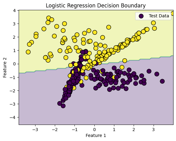
Explanation:
- Dataset:
- We use
make_classificationto generate a synthetic dataset with two features and a binary target variable (0or1).
- We use
- Logistic Regression Model:
- We initialize the logistic regression model using
LogisticRegression()fromsklearn. - The model is trained on the training data (
X_train,y_train), whereX_trainare the features andy_trainis the target class.
- We initialize the logistic regression model using
- Prediction and Evaluation:
- After training, we make predictions on the test data (
X_test). - We calculate the accuracy of the model by comparing the predicted values (
y_pred) with the actual values (y_test).
- After training, we make predictions on the test data (
- Visualization:
- The decision boundary is visualized using a contour plot, which shows the decision boundary between class 0 and class 1. The plot highlights how the logistic regression model separates the two classes based on the features.
Key Points:
- Logistic regression is widely used for binary classification (classifying data into two categories).
- The model provides the probability that a data point belongs to a certain class.
- The output is transformed using the sigmoid function, which is ideal for classification tasks with binary outcomes.
- It can be visualized by plotting the decision boundary and understanding how the model separates the classes.
Code Examples
Check out the Questions repo for the code used in this post and additional examples.