ernanhughes
+++ date = ‘2025-01-16T00:21:05Z’ title = ‘Cellular Automata: Introduction’ categories = [‘ca’] tag = [‘ca’] +++
Summary
This page is the first in a series of posts about Cellular Automata.
I believe that we could get the first evidence of AI through cellular automata.
A recent paper Intelligence at the Edge of Chaos found that LLM’s trained on more complex data generate better results. Which makes sense in a human context like the harder the material is I study the smarter I get. We need to find out why this is also the case with machines. The conjecture of this paper is that creating intelligence may require only exposure to complexity.
There are some properties of Cellular Automata that I believe make them contenders for early emergence.
- Simple to Complex we see really simple constructions generating complex patterns.
- Mimics reality the patterns we generate very closly mimices patters we see in crystals. Crystals are dead but have a life like action maybe this is a simple pre life system. We can model this in CA.
- Similar to life patterns we see similar mathematical patters in how plants grow, insects reproduce.
By the end of this series we will know a lot more about Cellular Automata and hopefully why they apprear to be intelligent.
What Are Cellular Automata?
Cellular automata(CA) are mathematical model that consist of a grid of cells, where each cell can be in one of a finite number of states. These states evolve over time according to simple rules based on the states of neighboring cells.
Components of Cellular Automata:
Key Concepts
- Cells: The fundamental units of a CA, arranged in a regular grid. Each cell has a state, which can be binary (e.g., on/off) or take on multiple values.
- Grid: The system is usually represented as a grid, which can be:
– 1D: A single row of cells.
– 2D: A grid of rows and columns (e.g., like a chessboard).
– 3D: Analogous to 2D but extends to neighbors in all spatial dimensions.
– Higher dimensions are also possible but less common. - Neighborhood: The set of cells surrounding a given cell that influence its state during each time step. Common neighborhoods include the Moore neighborhood (8 surrounding cells) and the von Neumann neighborhood (4 directly adjacent cells).
- Update Rules: define the transition function that maps the current configuration of a cell and its neighbors to a new state. For a given state and neighborhood the rule specifies a single (deteministic) or a set of probabilities (probabilistic) new state.
- States: Each cell can have a state, like:
– Binary: On/Off, Alive/Dead (e.g., 0 or 1).
– Multi-state: A set of possible states (e.g., 0, 1, 2). - Time Steps: The system evolves in discrete time steps, applying the rules to all cells simultaneously.
Why Are Cellular Automata Interesting?
- Simple to Complex: Even with simple rules, cellular automata can produce highly complex patterns and behaviors.
- Applications: They are used in:
- Physics: Modeling fluid dynamics and crystal growth.
- Biology: Simulating ecosystems or the spread of diseases.
- Computer Science: Data compression and cryptography.
- Art: Generating patterns and procedural designs.
Types of Cellular Automata
There are various types of cellular automata, each with unique characteristics and applications:
- Elementary Cellular Automata (ECA): The simplest class of CA with a one-dimensional grid, two possible cell states, and rules based on the state of the cell and its two immediate neighbors.
- Continuous Cellular Automata: CA where cell states can take on continuous values, allowing for smoother transitions and more nuanced behavior. Lenia is a notable example of this type.
- Neural Cellular Automata (NCA): A more recent development where the update rules are implemented using artificial neural networks. This integration allows NCAs to learn and adapt their behavior based on data, enabling them to solve complex tasks like image recognition, shape generation, and even control problems.
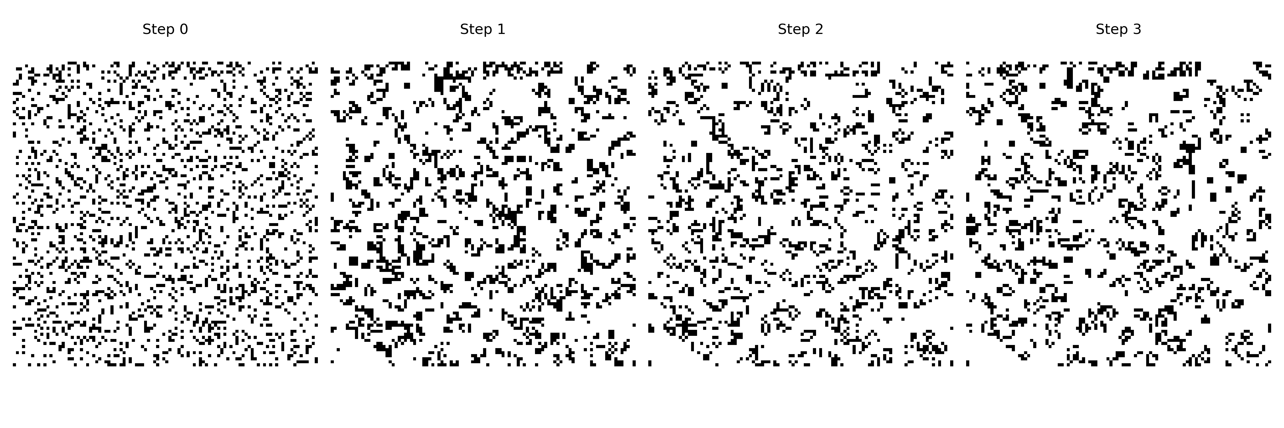
Conway’s Game of Life
The Game of Life demonstrates how complex and unpredictable patterns can arise from a set of very simple rules. This concept of emergence is fundamental to understanding how complex systems can arise from simple interactions. It bridges the gap between abstract computation (theoretical computer science) and physical systems.
Setup
- Grid: 2D grid.
- States: Each cell is either alive (1) or dead (0).
- Rules:
- A live cell with 2 or 3 live neighbors stays alive.
- A dead cell with exactly 3 live neighbors becomes alive.
- All other cells die or stay dead.
Despite these simple rules, it produces surprisingly complex and lifelike patterns.
import numpy as np
import matplotlib.pyplot as plt

# Constants
N = 100  # Grid size
ON = 255  # Value for live cells
OFF = 0  # Value for dead cells
NUM_SNAPSHOTS = 4  # Number of snapshots to display
OUTPUT_FILENAME = "game_of_life_snapshots.png"  # File name for the PNG

# Initialize grid with random on/off values
def initialize_grid(size, on_prob=0.2):
    return np.random.choice([ON, OFF], size * size, p=[on_prob, 1 - on_prob]).reshape(size, size)

# Compute the next state of the grid
def update_grid(grid):
    new_grid = grid.copy()
    for i in range(N):
        for j in range(N):
            # Compute the sum of the 8 neighbors using toroidal boundary conditions
            neighbors = (
                grid[i, (j - 1) % N] + grid[i, (j + 1) % N] +
                grid[(i - 1) % N, j] + grid[(i + 1) % N, j] +
                grid[(i - 1) % N, (j - 1) % N] + grid[(i - 1) % N, (j + 1) % N] +
                grid[(i + 1) % N, (j - 1) % N] + grid[(i + 1) % N, (j + 1) % N]
            ) / 255

            # Apply Conway's rules
            if grid[i, j] == ON:
                if neighbors < 2 or neighbors > 3:
                    new_grid[i, j] = OFF
            else:
                if neighbors == 3:
                    new_grid[i, j] = ON
    return new_grid

# Generate multiple snapshots of the grid
def generate_snapshots(grid, num_steps):
    snapshots = [grid]
    for _ in range(num_steps - 1):
        grid = update_grid(grid)
        snapshots.append(grid)
    return snapshots

# Plot snapshots side by side and save as PNG
def plot_snapshots(snapshots, output_filename=None):
    num_snapshots = len(snapshots)
    fig, axes = plt.subplots(1, num_snapshots, figsize=(15, 5))

    for i, ax in enumerate(axes):
        ax.matshow(snapshots[i], cmap="binary")
        ax.set_title(f"Step {i}")
        ax.axis("off")
1d Cellular Automata
Setup
A 1D cellular automaton consists of:
- A row of cells: Each cell is part of a linear array.
- Discrete states: Each cell can take on a finite set of states, typically
0or1in binary systems. - Discrete time steps: The system evolves in discrete steps, with all cells updating their states simultaneously.
- Neighborhood: Each cell’s new state depends on its current state and the states of its immediate neighbors.
Rules
1. The Neighborhood
- Radius: The radius defines how many neighbors on either side of a cell are considered. For most 1D CAs, a radius of 1 is used, meaning each cell is influenced by its immediate left and right neighbors.
-
Neighborhood Size: For a radius-1 neighborhood, the total number of cells influencing the state of a cell is:
[ \text{Neighborhood Size} = 2 \times \text{Radius} + 1 ]
So, with a radius of 1, the neighborhood size is 3 (left neighbor, the cell itself, and the right neighbor).
2. Total Number of Configurations
For binary states (0 or 1), the number of possible configurations of a neighborhood is:
[ 2^{\text{Neighborhood Size}} = 2^3 = 8 ]
Each configuration maps to a new state (0 or 1), leading to (2^8 = 256) possible rules for a radius-1, binary-state 1D cellular automaton.
3. Rule Representation
Rules are often represented as a binary sequence corresponding to all possible neighborhood configurations. For example, in Rule 30:
| Neighborhood | 111 | 110 | 101 | 100 | 011 | 010 | 001 | 000 |
|---|---|---|---|---|---|---|---|---|
| New State | 0 | 0 | 0 | 1 | 1 | 1 | 1 | 0 |
This rule is encoded as 00011110 in binary or as 30 in decimal (hence the name Rule 30).
Examples of 1D Cellular Automata Rules
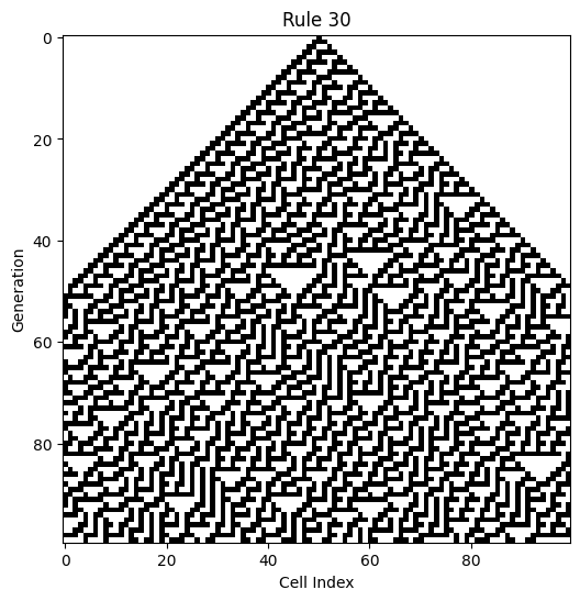
Rule 30
Rule 30 is one of the most famous 1D CA rules, known for its chaotic, unpredictable patterns despite its simple definition. It has been used in random number generation and even cryptography.
- Behavior: Starting with a single active cell, Rule 30 produces a triangular, fractal-like pattern with a mix of order and chaos.
- Emergent Complexity: This rule shows how deterministic local interactions can create highly intricate global structures.
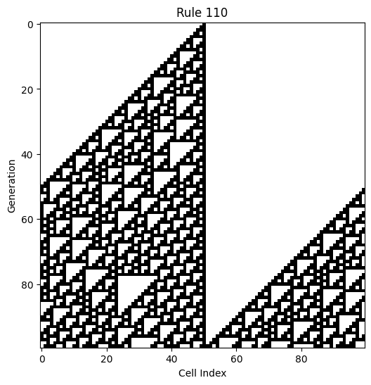
Rule 110
Rule 110 is particularly significant because it is Turing complete, meaning it can simulate any computation that a Turing machine can perform.
- Behavior: Rule 110 produces a mix of stable structures, moving patterns, and chaotic regions, making it an excellent example of emergent behavior.
- Importance: Its Turing completeness demonstrates that even simple systems can achieve universal computation.
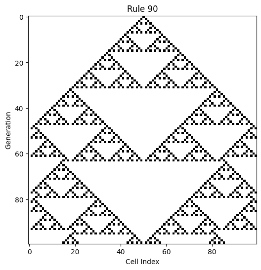
Rule 90
Rule 90 generates a well-known Sierpiński triangle pattern.
- Behavior: Each cell’s state is the XOR (exclusive OR) of its two neighbors’ states.
- Applications: Rule 90 is used to illustrate self-similarity and fractal structures in computational systems.
<img src="" width="" height="" alt="">
Class to support generation and display of all 1D rules
This class will support genrating and disaplaying all 1D rules 0 -255
import numpy as np
import matplotlib.pyplot as plt
from ipywidgets import interact, IntSlider
from IPython.display import display

class CellularAutomaton1D:
    def __init__(self, rule_number, size=100, steps=100, init_cond='single'):
        self.rule_number = rule_number  # Rule number (0-255)
        self.size = size                # Number of cells in a generation
        self.steps = steps              # Number of generations to simulate
        self.init_cond = init_cond      # Initial condition ('single', 'random', or custom array)
        self.rule_binary = np.array(self._decimal_to_binary(rule_number))
        self.grid = np.zeros((steps, size), dtype=np.int8)
        self.current_generation = np.zeros(size, dtype=np.int8)
        self._init_first_generation()

    def _decimal_to_binary(self, n):
        """Convert a decimal number to an 8-bit binary representation."""
        return np.array([int(x) for x in np.binary_repr(n, width=8)])

    def _init_first_generation(self):
        """Initialize the first generation based on the initial condition."""
        if self.init_cond == 'single':
            # Single cell in the middle set to 1
            self.current_generation[self.size // 2] = 1
        elif self.init_cond == 'random':
            # Random initial state
            self.current_generation = np.random.choice([0, 1], size=self.size)
        elif isinstance(self.init_cond, np.ndarray) and len(self.init_cond) == self.size:
            # Custom initial state provided as an array
            self.current_generation = self.init_cond.copy()
        else:
            raise ValueError("Invalid initial condition.")
        self.grid[0] = self.current_generation.copy()

    def _get_neighborhood(self, i):
        """Get the neighborhood of cell i with periodic boundary conditions."""
        left = self.current_generation[(i - 1) % self.size]
        center = self.current_generation[i]
        right = self.current_generation[(i + 1) % self.size]
        return left, center, right

    def _apply_rule(self, neighborhood):
        """Determine the new state of a cell based on its neighborhood and the rule."""
        # Convert the neighborhood to an index (0-7)
        idx = 7 - int(''.join(str(bit) for bit in neighborhood), 2)
        return self.rule_binary[idx]

    def run(self):
        """Run the cellular automaton simulation."""
        for step in range(1, self.steps):
            new_generation = np.zeros(self.size, dtype=np.int8)
            for i in range(self.size):
                neighborhood = self._get_neighborhood(i)
                new_state = self._apply_rule(neighborhood)
                new_generation[i] = new_state
            self.current_generation = new_generation
            self.grid[step] = self.current_generation.copy()

    def get_grid(self):
        return self.grid

    def display(self):
        """Display the simulation results."""
        plt.figure(figsize=(12, 6))
        plt.imshow(self.grid, cmap='binary', interpolation='nearest')
        plt.title(f'Rule {self.rule_number}')
        plt.xlabel('Cell Index')
        plt.ylabel('Generation')
        plt.show()
Display all rules
These functions will generate all the rules and display them as an image
def generate_all_automata(size=40, steps=40, init_cond='single'):
    automata_grids = []
    for rule_number in range(256):
        ca = CellularAutomaton1D(rule_number=rule_number, size=size, steps=steps, init_cond=init_cond)
        ca.run()
        grid = ca.get_grid()
        automata_grids.append(grid)
    return automata_grids


def display_all_automata(automata_grids, items_per_row=10, output_filename="all_rules.png"):
    total_automata = len(automata_grids)
    num_rows = total_automata // items_per_row
    if total_automata % items_per_row != 0:
        num_rows += 1

    fig, axes = plt.subplots(num_rows, items_per_row, figsize=(items_per_row * 1.5, num_rows * 1.5))
    # Increase hspace to add more vertical space between rows
    plt.subplots_adjust(wspace=0.1, hspace=0.5)

    for idx, grid in enumerate(automata_grids):
        row = idx // items_per_row
        col = idx % items_per_row
        if num_rows > 1:
            ax = axes[row, col]
        else:
            ax = axes[col]
        ax.imshow(grid, cmap='binary', interpolation='nearest')
        ax.set_title(f'Rule {idx}', fontsize=8)
        ax.axis('off')

    # Hide any unused subplots
    for idx in range(total_automata, num_rows * items_per_row):
        row = idx // items_per_row
        col = idx % items_per_row
        if num_rows > 1:
            ax = axes[row, col]
        else:
            ax = axes[col]
        ax.axis('off')

    plt.savefig(output_filename, dpi=300)
    plt.show()

# Generate and display all automata
automata_grids = generate_all_automata(size=100, steps=100, init_cond='single')
display_all_automata(automata_grids, items_per_row=8)
Code Examples
Check out the ca notebooks for the code used in this post and additional examples.